
Artificial Neural Network Basics#
Neural networks#
An artifical neural network mimics the action of neurons in your brain to form connections between nodes (neurons) that link the input to the output.
Note
We’ll loosely follow the notation from Computational Methods for Physics by Franklin.
Basic idea:
Create a nonlinear fitting routine with free parameters
Train the network on data with known inputs and outputs to set the parameters
Use the trained network on new data to predict the outcome
We can think of a neural network as a map that takes a set of \(N_\mathrm{in}\) parameters and returns a set of \(N_\mathrm{out}\) parameters, which we can express this as:
where
are the inputs,
are the outputs, and \({\bf A}\) is an \(N_\mathrm{out} \times N_\mathrm{in}\) matrix.
Our goal is to determine the matrix elements of \({\bf A}\).
Nomenclature#
We can visualize a neural network as:
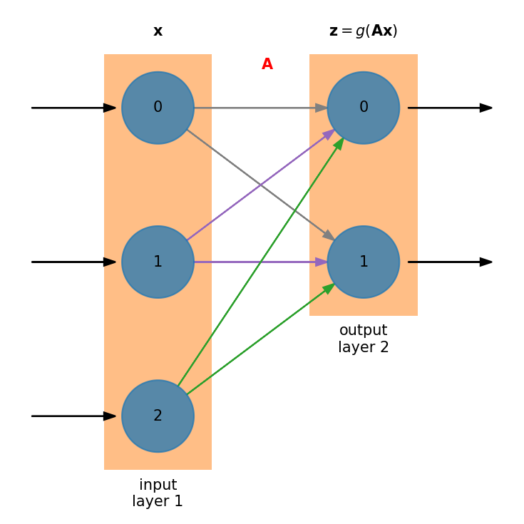
Neural networks are divided into layers
There is always an input layer—it doesn’t do any processing.
There is always an output layer.
Within a layer there are neurons or nodes.
For input, there will be one node for each input variable. In this figure, there are 3 nodes on the input layer.
The output layer will have as many nodes are needed to convey the answer we are seeking from the network. In this case, there are 2 nodes on the output layer.
Every node in the first layer connects to every node in the next layer
The weight associated with the connection can vary—these are the matrix elements.
Note
This is called a dense layer. There are alternate types of layers we can explore where the nodes are connected differently.
In this example, the processing is done in layer 2 (the output)
When you train the neural network, you are adjusting the weights connecting to the nodes
Some connections might have zero weight
This mimics nature—a single neuron can connect to several (or lots) of other neurons.
Universal approximation theorem#
A neural network can be designed to approximate any function, \(f(x)\). For this to work, there must be a source of non-linearity in the network—this is a result of the universal approximation theorem.
We use a nonlinear activation function that is applied in a layer. It has the form:
Note
The activation function, \(g({\bf v})\) works element-by-element on the vector \({\bf v}\).
Then our neural network has the form: \({\bf z} = g({\bf A x})\)
We want to choose a function \(g(\xi)\) that is differentiable. A common choice is the sigmoid function:
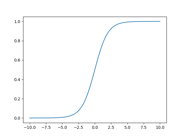
Fig. 9 The sigmoid function#
Note
There are many choices for the activation function which have different properties. Often the choice of activation function will be empirical, by experimenting with the performance of the network.
Basic algorithm#
We’ll consider the case where we have training data—a set of inputs, \({\bf x}^k\), together with the expected output (answer), \({\bf y}^k\). These training pairs allow us to constrain the output of the network and train the weights.
Training
Loop over the \(T\) pairs \(({\bf x}^k, {\bf y}^k)\) for \(k = 1, \ldots, T\)
Predict the output for \({\bf x}^k\) as:
\[z_i = g([{\bf A x}^k]_i) = g \left ( \sum_{j=1}^{N_\mathrm{in}} A_{ij} x^k_j \right )\]Constrain that \({\bf z} = {\bf y}^k\).
This is a minimization problem, where we are minimizing:
\[\begin{align*} \mathcal{L}(A_{ij}) &= \| g({\bf A x}^k) - {\bf y}^k \|^2 \\ &= \sum_{i=1}^{N_\mathrm{out}} \left [ g\left (\sum_{j=1}^{N_\mathrm{in}} A_{ij} x^k_j \right ) - y^k_i \right ]^2 \end{align*}\]We call this function, \(\mathcal{L}\), the cost function or loss function.
Note
This is called the mean square error loss function, and is one possible choice for \(\mathcal{L}(A_{ij})\), but many others exist.
Update the matrix \({\bf A}\) based on the training pair \(({\bf x}^k, {\bf y^{k}})\).
Using the network
With the trained \({\bf A}\), we can now use the network on data we haven’t seen before, \(\boldsymbol \chi\):
\[z_i = g([{\bf A {\boldsymbol \chi}}^k]_i) = g \left ( \sum_{j=1}^{N_\mathrm{in}} A_{ij} \chi^k_j \right )\]
There are a lot of details that we still need to figure out involving the training and minimization. We’ll start with minimization: a common minimization technique used with neural networks is gradient descent.