Two Point Boundary Value Problems

Consider a Poisson equation:

\[u^{\prime\prime} = f(x, u)\]

on \([0, 1]\). This is a second-order ODE, so it requires 2 boundary conditions. Let’s take:

\[\begin{align*} u(0) &= a \\ u(1) &= b \end{align*}\]

Important

These boundary conditions are at opposite ends on the domain—this is not an initial value problem. The methods we used thus far do not work on this.

We’d like to turn this into an initial value problem so we can reuse the methods we already developed (like 4th-order Runge-Kutta). We’ll see here how we can do this. via the shooting method.

Note

Later we’ll see how to apply relaxation methods to this problem.

Shooting

Let’s rewrite this as a system defining:

\[\begin{align*} y &= u \\ z &= u^\prime \end{align*}\]

Let’s take the left boundary conditions as:

\[\begin{align*} y(0) &= a \\ z(0) &= \eta \end{align*}\]

Important

What is \(\eta\)? This is a parameter that we will adjust to make the solution yield \(y(1) = b\) at the end of integration. We’ll call the solution for a particular value of \(\eta\): \(y^{(\eta)}(x)\).

Shooting algorithm:

• Guess \(\eta\)

• Iterate:

  • Integrate system to right boundary

  • Use secant method to zero \(f(\eta) = b - y^{(\eta)}(1)\)

  • Correct \(\eta\)

First example

Consider:

\[u^{\prime\prime} = \sin(x)\]

with

\[\begin{align*} u(0) &= 0 \\ u(1) &= 1 \end{align*}\]

Note

This is a linear ODE, since \(u\) only appears linearly in the equation.

We can integrate this twice and find:

\[u(x) = -\sin(x) + c_1 x + c_2\]

where \(c_1\) and \(c_2\) are integration constants. Applying the boundary conditions, we get:

\[u(x) = -\sin(x) + (1 + \sin(1)) x\]

Rewriting this system, we have:

\[\begin{align*} y^\prime &= z \\ z^\prime &= \sin(x) \end{align*}\]

Here’s an implementation that uses RK4.

First the RHS function:

import numpy as np
import matplotlib.pyplot as plt

def rhs(x, y, z):
    """ RHS function.  Here y = u, z = u'"""
    
    dydx = z
    dzdx = np.sin(x)

    return dydx, dzdx

Now a simple fixed-stepsize RK4 integrator:

def rk4(y0, eta0, rhs, xl=0.0, xr=1.0, n=100):
    """
    R-K 4 integration: y0 and eta0 are y(0) and z(0); rhs is the
    righthand side function xl and xr are the domain limits n
    is the number of integration points (including starting point)

    """
    
    # compute the step size
    h = (xr - xl) / (n - 1)

    y = np.zeros(n)
    z = np.zeros(n)

    # left boundary initialization
    y[0] = y0
    z[0] = eta0

    x = xl
    for m in range(n-1):
        dydx_1, dzdx_1 = rhs(x, y[m], z[m])
        dydx_2, dzdx_2 = rhs(x + 0.5 * h, y[m] + 0.5 * h * dydx_1, z[m] + 0.5 * h * dzdx_1)
        dydx_3, dzdx_3 = rhs(x + 0.5 * h, y[m] + 0.5 * h * dydx_2, z[m] + 0.5 * h * dzdx_2)
        dydx_4, dzdx_4 = rhs(x + h, y[m] + h * dydx_3, z[m] + h * dzdx_3)

        y[m+1] = y[m] + (h / 6.0) * (dydx_1 + 2.0 * dydx_2 + 2.0 * dydx_3 + dydx_4)
        z[m+1] = z[m] + (h / 6.0) * (dzdx_1 + 2.0 * dzdx_2 + 2.0 * dzdx_3 + dzdx_4)

        x += h
    return y, z

and finally the driver. Here we specify the right boundary condition (\(b\)) via the parameter y_right_true. Also note that if we pass in a matplotlib Axis object via ax, we’ll plot the progress as we iterate.

def solve_bvp(npts, rhs, *,
              xl=0, xr=1,
              y_right_true=1, eps=1.e-8, ax=None):
    
    """shoot from x = 0 to x = 1.  We will do this by selecting a boundary
    value for z and use a secant method to adjust it until we reach the
    desired boundary condition at y(1)"""

    # initial guess
    y_0 = 0.0   # this is the correct boundary condition a x = 0
    eta = 0.0   # this is what we will adjust to get the desired y1(1)

    # Secant loop
    dy = 1.e30    # fail first time through

    # keep track of iteration for plotting
    iter = 0

    while dy > eps:
        # integrate
        y, z = rk4(y_0, eta, rhs, xl=0.0, xr=1.0, n=npts)

        if ax:
            x = np.linspace(xl, xr, npts)
            ax.scatter(x, y, label=f"iteration {iter}", marker="x")

        if iter == 0:
            # we don't yet have enough information to estimate
            # the derivative.  So store what we have and
            # go to the next iteration
            eta_m1 = eta
            eta = -1
            y_old = y
            iter += 1
            continue
            
        # do a Secant method to correct.  Here eta = y2(0) -- our
        # control parameter.  We want to zero:
        #   f(eta) = y1_true(1) - y1^(eta)(1)

        # derivative (for Secant)
        dfdeta = ( (y_right_true - y_old[-1]) -
                   (y_right_true - y[-1]) ) / (eta_m1 - eta)

        # correction by f(eta) = 0 = f(eta_0) + dfdeta deta
        deta = -(y_right_true - y[-1]) / dfdeta

        # store the old guess and correct
        eta_m1 = eta
        eta += deta

        dy = abs(deta)

        y_old = y

        iter += 1
        print(f"finished iter {iter}, error = {dy}")
        
    return eta, y, z

Now we’ll run it, making plots along the way. We’ll also show the analytic solution

def analytic(x):
    """ analytic solution """
    return -np.sin(x) + (1.0 + np.sin(1)) * x

fig, ax = plt.subplots()

eta, y, z = solve_bvp(16, rhs, ax=ax)

x = np.linspace(0, 1, 100)
ax.plot(x, analytic(x), color="0.5", ls="-", label="analytic")
ax.legend()

finished iter 2, error = 1.841470960630243
finished iter 3, error = 0.0

<matplotlib.legend.Legend at 0x7f60108e23d0>

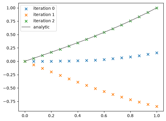
Notice that we get the correct solution after only 2 iterations—this is mainly because this is a linear problem.

Nonlinear example

Consider the problem:

\[u^{\prime\prime} + u^2 = -\sin(x) (1 - \sin(x))\]

on \([0, 1]\) with

\[\begin{align*} u(0) &= 0 \\ u(1) &= \sin(1) \end{align*}\]

Note

This is nonlinear because the term \(u^2\) appears in the equation.

This has the solution: \(u(x) = \sin(x)\)

Rewriting it in terms of \(y = u\) and \(z = u^\prime\), we have:

\[\begin{align*} y' &= z \\ z' &= -y^2 - \sin(x) (1 - \sin(x)) \end{align*}\]

Here’s the righthand side function for this new system

def rhs2(x, y, z):
    """ RHS function.  Here y = u, z = u'"""
    
    dydx = z
    dzdx = -y**2 - np.sin(x) * (1.0 - np.sin(x))

    return dydx, dzdx

and the analytic solution

def analytic2(x):
    """ analytic solution """
    return np.sin(x)

fig, ax = plt.subplots()

eta, y, z = solve_bvp(16, rhs2, ax=ax, y_right_true=np.sin(1))

x = np.linspace(0, 1, 100)
ax.plot(x, analytic2(x), color="0.5", ls="-", label="analytic")
ax.legend()

finished iter 2, error = 1.8466767840805172
finished iter 3, error = 0.12915051105171896
finished iter 4, error = 0.023858013890531087
finished iter 5, error = 0.00031404043908051616
finished iter 6, error = 6.497196603636414e-07
finished iter 7, error = 1.748051261871642e-11

<matplotlib.legend.Legend at 0x7f60103cb490>

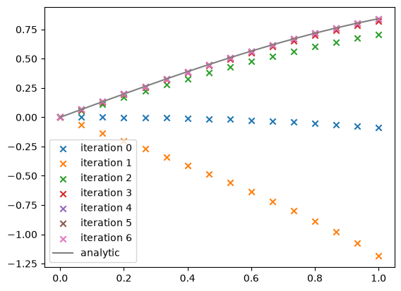
Now we see that it takes more iterations, but still converges.