Homework 2 solutions

We want to integrate the Planck function with a filter transmission profile to get a flux through the filter and then compute colors for stars.

Specifically, we want to do:

\[f_X \approx \int_0^\infty B_\lambda(T) s_X(\lambda) d\lambda\]

and then

\[B - V = -2.5 \log_{10}(f_B/f_V)\]

where our filter is just a step function:

\[\begin{split}s_X(\lambda) = \left \{ \begin{array}{cc} 1 & |\lambda - \lambda_{0,X}| \le \frac{d\lambda_X}{2} \\ 0 & \mbox{otherwise} \end{array} \right . \end{split}\]

import numpy as np
import matplotlib.pyplot as plt

Let’s start by defining the Planck function. We’ll work in CGS units (unlike in class where we made this dimensionless).

def B(lam, T=1.e4):
    """Planck function.  Here lambda is wavelength in cm,
    T is temperature in K"""
    k = 1.38e-16
    h = 6.63e-27
    c = 3.e10
    # we need to take the limit x -> 0 if the input x is 0
    return np.where(lam == 0, 0,
                    2 * h * c**2 / lam**5 / np.expm1(h*c/(lam*k*T)))

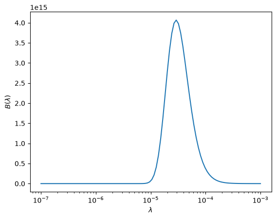
Let’s just make sure that our \(B(\lambda)\) looks like it should. For \(T = 10^4~\mathrm{K}\), it should peak in the visible.

fig, ax = plt.subplots()
T = 1.e4
lam = np.logspace(-7, -3, 100)
ax.plot(lam, B(lam, T))
ax.set_xscale("log")
ax.set_xlabel(r"$\lambda$")
ax.set_ylabel(r"$B(\lambda)$")

/tmp/ipykernel_4601/55925149.py:9: RuntimeWarning: overflow encountered in expm1
  2 * h * c**2 / lam**5 / np.expm1(h*c/(lam*k*T)))

Text(0, 0.5, '$B(\\lambda)$')

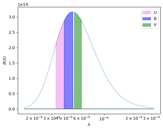
Now let’s define the filters (I’ll include U here for fun). This stores \(\lambda_0\) and \(d\lambda\) for each filter in a dict keyed on the filter name.

filters = {"U": (365e-7, 70e-7),
           "B": (445e-7, 90e-7),
           "V": (550e-7, 90e-7)}

Next, we’ll write a function that computes the filter’s response.

def filter_response(lam, lambda0, dlambda=50e-7):
    return np.where(np.logical_and(lam > lambda0-0.5*dlambda,
                                   lam < lambda0+0.5*dlambda), 1.0, 0.0)

and then a function that combines the filter and the Planck function — this will be our integrand.

Note

I use a * here on the tuple that holds the filter parameters—this is an example of the python unpacking operator.

def filtered_B(lam, T=1.e4, filter="B"):
    return B(lam, T=T) * filter_response(lam, *filters[filter])

Now let’s plot this filtered Planck function to see what it looks like.

T = 6000

lam = np.logspace(-4.8, -3.5, 1000)

fig, ax = plt.subplots()

ax.fill(lam, filtered_B(lam, T=T, filter="U"),
        label="U", color="violet", alpha=0.5)
ax.fill(lam, filtered_B(lam, T=T, filter="B"),
        label="B", color="blue", alpha=0.5)
ax.fill(lam, filtered_B(lam, T=T, filter="V"),
        label="V", color="green", alpha=0.5)

ax.plot(lam, B(lam, T=T), ls=":")

ax.set_xscale("log")
ax.set_xlabel(r"$\lambda$")
ax.set_ylabel(r"$B(\lambda)$")
ax.legend()

<matplotlib.legend.Legend at 0x7fc11ed3d1d0>

We have different options for doing the integrals. Since our \(s(x)\) is just a step function, we actually need to just integrate:

\[f_X \approx \int_{\lambda_{0,X} - d\lambda_X/2}^{\lambda_{0,X} + d\lambda_X/2} B_\lambda(T) s_X(\lambda) d\lambda\]

so we don’t need to use the machinery we developed in class for dealing with integrals to \(\infty\).

I’ll still use that here though, just because we might want to consider a different filter someday…

Let’s define the transform functions and a composite trapezoid rule that works with them:

SMALL = 1.e-30

def zv(x, alpha=1):
    """ transform the variable x -> z """
    return x/(alpha + x) 

def xv(z, alpha=1):
    """ transform back from z -> x """
    return alpha*z/(1.0 - z + SMALL)

def I_t(func, N=10, alpha=5, args=None):
    """composite trapezoid rule for integrating from [0, oo].
    Here N is the number of intervals"""

    if args is None:
        args = ()
        
    # there are N+1 points corresponding to N intervals
    z = np.linspace(0.0, 1.0, N+1, endpoint=True)
    
    I = 0.0
    for n in range(N):
        I += 0.5 * ((z[n+1] - z[n]) *
                    (func(xv(z[n], alpha), *args) / (1.0 - z[n] + SMALL)**2 +
                     func(xv(z[n+1], alpha), *args) / (1.0 - z[n+1] + SMALL)**2))
    I *= alpha
    return I

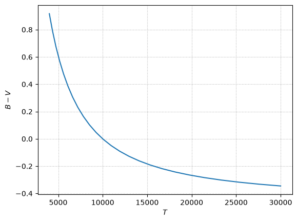
Now, we want to compute the zero-point of \(B-V\) as that of a \(T = 10^4~\mathrm{K}\) star. We’ll call this BV0:

T = 10000
BV0 = -2.5*np.log10(I_t(filtered_B, N=250,
                        alpha=filters["B"][0], args=(T, "B")) /
                    I_t(filtered_B, N=250,
                        alpha=filters["V"][0], args=(T, "V")))

/tmp/ipykernel_4601/55925149.py:9: RuntimeWarning: divide by zero encountered in scalar divide
  2 * h * c**2 / lam**5 / np.expm1(h*c/(lam*k*T)))
/tmp/ipykernel_4601/55925149.py:9: RuntimeWarning: invalid value encountered in scalar divide
  2 * h * c**2 / lam**5 / np.expm1(h*c/(lam*k*T)))
/tmp/ipykernel_4601/55925149.py:9: RuntimeWarning: overflow encountered in expm1
  2 * h * c**2 / lam**5 / np.expm1(h*c/(lam*k*T)))

Finally, let’s compute all of the \(B-V\) for different \(T\), making sure to correct with BV0:

Ts = np.logspace(np.log10(4000), np.log10(30000), 25)
BVs = []

for T in Ts:
    BV = -2.5*np.log10(I_t(filtered_B, N=250,
                           alpha=filters["B"][0], args=(T, "B")) /
                       I_t(filtered_B, N=250,
                           alpha=filters["V"][0], args=(T, "V"))) - BV0
    BVs.append(BV)

/tmp/ipykernel_4601/55925149.py:9: RuntimeWarning: divide by zero encountered in scalar divide
  2 * h * c**2 / lam**5 / np.expm1(h*c/(lam*k*T)))
/tmp/ipykernel_4601/55925149.py:9: RuntimeWarning: invalid value encountered in scalar divide
  2 * h * c**2 / lam**5 / np.expm1(h*c/(lam*k*T)))
/tmp/ipykernel_4601/55925149.py:9: RuntimeWarning: overflow encountered in expm1
  2 * h * c**2 / lam**5 / np.expm1(h*c/(lam*k*T)))

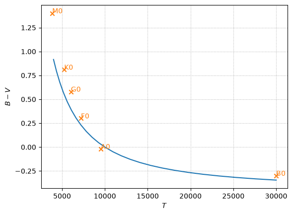
fig, ax = plt.subplots()
ax.plot(Ts, BVs)
ax.grid(ls=":")
ax.set_xlabel("$T$")
ax.set_ylabel("$B-V$")

Text(0, 0.5, '$B-V$')

and we’ll add points for real stars

stars = [("B0", 30000, -0.30),
         ("A0", 9520, -0.02),
         ("F0", 7200, +0.30),
         ("G0", 6030, +0.58),
         ("K0", 5250, +0.81),
         ("M0", 3850, +1.40)]

for l, T, BV in stars:
    ax.scatter(T, BV, marker="x", color="C1")
    ax.text(T, BV, l, color="C1")
fig

Caution

You may have thought that you could just use scipy.integrate.quad to do the integration from \([0, \infty]\), but it doesn’t get the right answer.

from scipy import integrate
T = 1.e4
I, err = integrate.quad(filtered_B, 0, np.inf, args=(T, "B"))
I

0.0

The issue here is that our integrand peaks at \(\lambda \sim 10^{-5}~\mathrm{cm}\) and the quad() function simply does not notice this. We should instead make the integrand dimensionless so the peak is near 1. We accomplished this manually with our choice of \(\alpha\) in our method.

We can get do better if we restrict the integration limits

I, err = integrate.quad(filtered_B, 5.e-6, 2.e-4,
                        limit=100, args=(T, "B"))
I

25172574924.317474

But we really need to make the integrand dimensionless to get the best result here.