
Going Further#
Cubic splines#
Cubic splines are a popular way of interpolating data. A cubic polynomial is fit to 2 adjacent data samples. Consider a cubic of the form:
We want to fit \(p_i(x)\) to the range \([x_i, x_{i+1}]\), as illustrated here:
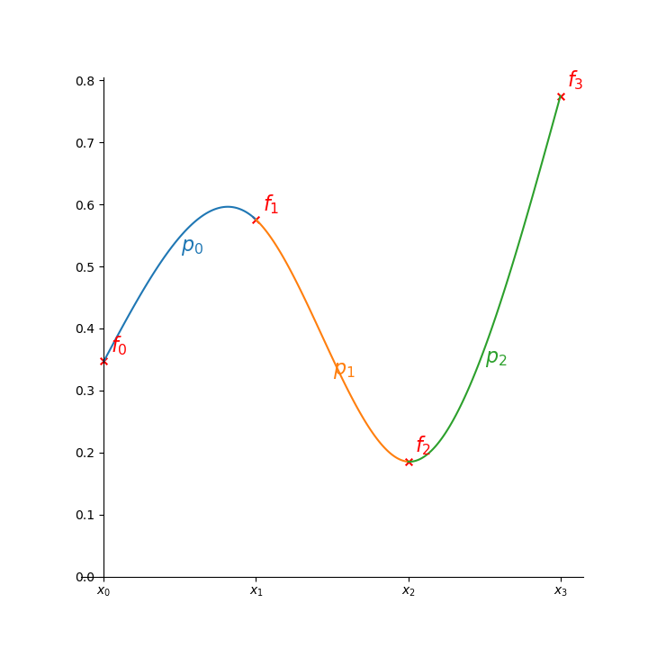
Consider the points \((x_1, f_1)\) and \((x_2, f_2)\). Since we need 4 parameters to fit a cubic, we use the values of the function at the two points as well as the derivatives. And the derivatives of the cubic at the end point are matched to those of the next cubic spline.
At \(x_1\):
\(p_0(x_1) = f_1\)
\(p_1(x_1) = f_1\)
\(p_0^\prime(x_1) = p_1^\prime(x_1)\)
\(p_0^{\prime\prime}(x_1) = p_1^{\prime\prime}(x_1)\)
and at \(x_2\):
\(p_1(x_2) = f_2\)
\(p_2(x_2) = f_2\)
\(p_1^\prime(x_2) = p_2^\prime(x_2)\)
\(p_1^{\prime\prime}(x_2) = p_2^{\prime\prime}(x_2)\)
This means that all of the cubics are coupled together, and a linear system needs to be solved for find all of the coefficients simultaneously.
Thermodynamic consistency#
One place where interpolation is widely used in astrophysics is in interpolating complex equations of state (like electron degeneracy) where computing the functions is very computationally expensive. By creating a grid of \(\rho, T\) points where the results are tabulated, a high-order, multidimensional interpolant can be used to cheaply find the thermodynamic state.
However, care must be taken to ensure that the results are thermodynamically consistent. This is discussed in the paper The Accuracy, Consistency, and Speed of an Electron-Positron Equation of State Based on Table Interpolation of the Helmholtz Free Energy.