
Galaxy Classification with a Neural Net from Scratch#
Here we implement a neural network from scratch with a single hidden layer, using only NumPy and use it to classify galaxies.
import numpy as np
import matplotlib.pyplot as plt
import h5py
We need the Galaxy class we previously defined
galaxy_types = {0: "disturbed galaxies",
                1: "merging galaxies",
                2: "round smooth galaxies",
                3: "in-between round smooth galaxies",
                4: "cigar shaped smooth galaxies",
                5: "barred spiral galaxies",
                6: "unbarred tight spiral galaxies",
                7: "unbarred loose spiral galaxies",
                8: "edge-on galaxies without bulge",
                9: "edge-on galaxies with bulge"}
class Galaxy:
    def __init__(self, data, answer, *, index=-1):
        self.data = np.array(data, dtype=np.float32) / 255.0 * 0.99 + 0.01
        self.answer = answer

        self.out = np.zeros(10, dtype=np.float32) + 0.01
        self.out[self.answer] = 0.99

        self.index = index

    def plot(self, ax=None):
        if ax is None:
            fig, ax = plt.subplots()
        ax.imshow(self.data, interpolation="nearest")
        ax.text(0.025, 0.95, f"answer: {self.answer}",
                color="white", transform=ax.transAxes)

    def validate(self, prediction):
        """check if a categorical prediction matches the answer"""
        return np.argmax(prediction) == self.answer
A manager class#
We’ll create a class to manage access to the data. This will do the following:
open the file and store the handles to access the data
partition the data into test and training sets
provide a means to shuffle the data
provide methods to get the next dataset (either training or test)
allow us to coarsen the images to a reduced resolution to reduce the memory requirements and make the training easier.
Tip
Since every input node is connected to every hidden layer node (a dense network), there are a lot of weights to train. By using smaller images, it is easier to train.
class DataManager:
    def __init__(self, partition=0.8,
                 datafile="Galaxy10_DECals.h5",
                 include_transformation=False,
                 coarsen=1):
        """manage access to the data

        partition: fraction that should be training
        datafile: name of the hdf5 file with the data
        coarsen: reduce the number of pixels by this factor
        """

        self.ds = h5py.File(datafile)
        self.ans = np.array(self.ds["ans"])
        self.images = np.array(self.ds["images"])

        self.coarsen = coarsen

        self.include_transformation = include_transformation

        N = len(self.ans)

        # create a set of indices for the galaxies and randomize
        self.indices = np.arange(N, dtype=np.uint32)
        self.rng = np.random.default_rng()
        self.rng.shuffle(self.indices)

        # partition into training and test sets
        # these indices will always refer to the index in the original
        # unsplit dataset
        n_cut = int(partition * N)
        self.training_indices = self.indices[0:n_cut]
        self.test_indices = self.indices[n_cut:N]

        self.n_training = len(self.training_indices)
        if self.include_transformation:
            self.n_training *= 2
        self.n_test = len(self.test_indices)

        self.input_size = np.ravel(self._get_galaxy(0).data).size

    def _get_galaxy(self, index):
        """return a numpy array containing a single galaxy image, coarsened
        if necessary by averaging"""
        _tmp = self.images[index, :, :, :]
        if self.coarsen > 1:
            _tmp = np.mean(_tmp.reshape(_tmp.shape[0]//self.coarsen, self.coarsen,
                                        _tmp.shape[1]//self.coarsen, self.coarsen,
                                        _tmp.shape[2]), axis=(1, 3))
        return _tmp

    def training_images(self):
        self.reset_training()
        for idx in self.training_indices:
            yield Galaxy(self._get_galaxy(idx), self.ans[idx], index=idx)
            if self.include_transformation:
                yield Galaxy(np.rot90(self._get_galaxy(idx), axes=(0, 1)),
                             self.ans[idx], index=idx)

    def reset_training(self):
        """prepare for the next epoch: shuffle the training data and
        reset the index to point to the start"""
        self.rng.shuffle(self.training_indices)

    def test_images(self):
        for idx in self.test_indices:
            yield Galaxy(self._get_galaxy(idx), self.ans[idx], index=idx)
Tip
The training_images() and testing_images() are generators (like range()), so we can iterate like:
d = DataManager()
for g in d.training_images():
    # do stuff with g
and g is only converted to 32-bit float as needed.
We can now work with the data as follows. Here we create a DataManager that will coarsen the images by a factor of 4 (so they will be 64x64 pixels with 3 colors).
d = DataManager(coarsen=4, include_transformation=True)
we can see how many images there are in the training and test sets
d.n_training, d.n_test
(28376, 3548)
We can then get the first few training galaxies and look at them. Note that with transformations enabled, the should be pairs with one rotated 90 degrees compared to the previous.
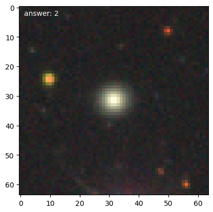
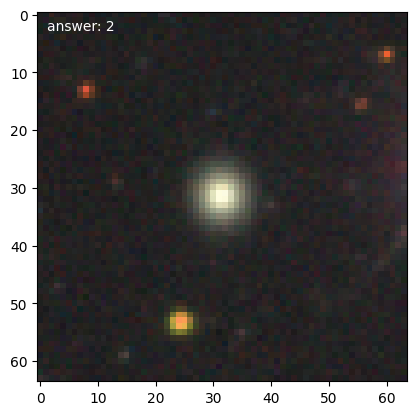
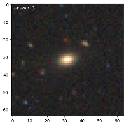
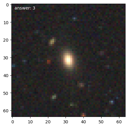
for n, g in enumerate(d.training_images()):
    g.plot()
    if n == 3:
        break
We’ll need a 1-d representation of the data, which the DataManager will provide
d.input_size
12288
Batching#
Training with this data will be very slow. We can speed it up more by using batching and aggregating the linear algebra. Here’s how this works.
Single input recap#
Our basic network does:
where the sizes of the matrices and vectors are:
\({\bf x}^k\) : \(N_\mathrm{in} \times 1\)
\({\bf B}\) : \(N_\mathrm{hidden} \times N_\mathrm{in}\)
\(\tilde{\bf z}^k\) : \(N_\mathrm{hidden}\times 1\)
\({\bf A}\) : \(N_\mathrm{out} \times N_\mathrm{hidden}\)
\({\bf z}^k\) : \(N_\mathrm{out} \times 1\)
we also have the known output, \({\bf y}^k\) corresponding to input \({\bf x}^k\)
\({\bf y}^k\) : \(N_\mathrm{out} \times 1\)
we then compute the errors:
\({\bf e}^k = {\bf z}^k - {\bf y}^k\) (the error on the output layer) : \(N_\mathrm{out} \times 1\)
\(\tilde{\bf e}^k = {\bf A}^\intercal \cdot [{\bf e}^k \circ {\bf z} \circ (1 - {\bf z})]\) (the error backpropagated to the hidden layer) : \(N_\mathrm{hidden} \times 1\)
and finally the corrections due to this single piece of training data, \(({\bf x}^k, {\bf y}^k)\):
\(\Delta {\bf A} = -2\eta \,{\bf e}^k \circ {\bf z}^k \circ (1 - {\bf z}^k) \cdot (\tilde{\bf z}^k)^\intercal\) : \(N_\mathrm{out} \times N_\mathrm{hidden}\)
\(\Delta {\bf B} = -2\eta \,\tilde{\bf e}^k \circ \tilde{\bf z}^k \circ (1 - \tilde{\bf z}^k) \cdot ({\bf x}^k)^\intercal\) : \(N_\mathrm{hidden} \times N_\mathrm{in}\)
A batching approach#
We now want to batch the inputs, by extending \({\bf x}\) to be of size \(N_\mathrm{in} \times S\), where \(S\) is the batch size. This means that each column is a unique input vector \({\bf x}^k\), and \(S\) of them are sandwiched together:
Similarly, we create a batched \({\bf y}_b\) that contains the \({\bf y}^k\) corresponding to the \({\bf x}^k\) in \({\bf x}_b\).
We can propagate this through the network, getting
where \({\bf z}_b\) is now of size \(N_\mathrm{out} \times S\).
Now, we compute the errors from the batched inputs
\({\bf e}_b = {\bf z}_b - {\bf y}_b\) : \(N_\mathrm{out} \times S\)
\(\tilde{\bf e}_b =\underbrace{{\bf A}^\intercal}_{N_\mathrm{hidden} \times N_\mathrm{out}} \cdot \underbrace{[{\bf e}_b \circ {\bf z}_b \circ (1 - {\bf z})]}_{N_\mathrm{out} \times S}\) : \(N_\mathrm{hidden} \times S\)
and the accumulated corrections:
\(\Delta {\bf A} = -\frac{2\eta}{S} \,\underbrace{{\bf e}_b \circ {\bf z}_b \circ (1 - {\bf z}_b)}_{N_\mathrm{out}\times S} \cdot \underbrace{(\tilde{\bf z}_b)^\intercal}_{S\times N_\mathrm{hidden}}\)
\(\Delta {\bf B} = -\frac{2\eta}{S} \,\underbrace{\tilde{\bf e}_b \circ \tilde{\bf z}_b \circ (1 - \tilde{\bf z}_b)}_{N_\mathrm{hidden} \times S} \cdot \underbrace{({\bf x}_b)^\intercal}_{S \times N_\mathrm{in}}\)
In these accumulated corrections, the \(S\) dimensions contract. In essence, this means that each element in \(\Delta {\bf A}\) and \(\Delta {\bf B}\) is the sum of the corrections for each of the \(S\) training data pairs in the batch. For this reason, we normalize by \(S\) to create the average of the gradient.
Tip
Batching also stabilizes the gradient descent, making it easier to find the minimum and allowing us to use a larger learning rate.
Momentum#
The other feature we need for this application is momentum in the gradient descent weight updates.
A popular form of momentum (see, e.g., Momentum: A simple, yet efficient optimizing technique) builds off of the idea of the exponential moving average.
For our gradient descent update, we usually do:
where \(\mathcal{L}\) is our loss function and \(\eta\) is the learning rate.
The basic idea of momentum begins with defining a “velocity”, \({\bf v}^{(0)} = 0\) (no momentum has been built up yet). Then each iteration of training we do the following:
construct the gradient from the current set of training, \(\partial \mathcal{L}/\partial {\bf A}\)
blend this with the previous momentum using an exponential moving average:
\[{\bf v}^{(i)} = \beta {\bf v}^{(i-1)} + (1 - \beta) \frac{\partial \mathcal{L}}{\partial {\bf A}}\]where \(\beta \in [0, 1]\) is the smoothing parameter. It seems like \(\beta = 0.9\) is used often.
Since every gradient is always multiplied by \((1-\beta)\), and each previous gradient picks up a factor of \(\beta\) each iteration, this construction weights the most recent gradients most.
update the weights:
\[{\bf A} = {\bf A} - \eta {\bf v}^{(i)}\]
We would do the same with the other weights, \({\bf B}\).
Tip
Momentum greatly reduces the swings in the “fraction correct” metric from one epoch to the next.
Implementing our neural network#
We’ll write our network to take a DataManager—it can get everything that it needs from there.
Tip
We also have our network do the validation against the test set each epoch so we can see how well we are doing.
import time
class NeuralNetwork:
    """A neural network class with a single hidden layer."""

    def __init__(self, data_manager, *, hidden_layer_size=20):

        self.data_manager = data_manager

        # the number of nodes/neurons on the output layer
        self.N_out = 10

        # the number of nodes/neurons on the input layer
        self.N_in = d.input_size

        # the number of nodes/neurons on the hidden layer
        self.N_hidden = hidden_layer_size

        # we will initialize the weights with Gaussian normal random
        # numbers centered on 0 with a width of 1/sqrt(n), where n is
        # the length of the input state
        rng = np.random.default_rng()

        # A is the set of weights between the hidden layer and output layer
        self.A = np.zeros((self.N_out, self.N_hidden), dtype=np.float32)
        self.A[:, :] = rng.normal(0.0, 1.0/np.sqrt(self.N_hidden), self.A.shape)

        # B is the set of weights between the input layer and hidden layer
        self.B = np.zeros((self.N_hidden, self.N_in), dtype=np.float32)
        self.B[:, :] = rng.normal(0.0, 1.0/np.sqrt(self.N_in), self.B.shape)

        # reset the training
        self.data_manager.reset_training()

        self.n_trained = 0
        self.training_time = 0

    def sigmoid(self, xi):
        """our sigmoid function that operates on the hidden layer"""
        return 1.0/(1.0 + np.exp(-xi))

    def _batch_update(self, x_batch, y_batch):

        # batch size
        S = len(x_batch)

        x = np.array(x_batch).T
        y = np.array(y_batch).T

        # propagate the input through the network
        z_tilde = self.sigmoid(self.B @ x)
        z = self.sigmoid(self.A @ z_tilde)

        # compute the errors (backpropagate to the hidden layer)
        e = z - y
        e_tilde = self.A.T @ (e * z * (1 - z))

        # corrections
        grad_A = (2/S) * e * z * (1 - z) @ z_tilde.T
        grad_B = (2/S) * e_tilde * z_tilde * (1 - z_tilde) @ x.T

        self.n_trained += S

        return grad_A, grad_B

    def assess(self):
        """Run through the test data and return the fraction correct
        with the currently trained network"""

        n_correct = 0
        for g in self.data_manager.test_images():
            ans = self.predict(g)
            if g.validate(ans):
                n_correct += 1

        return n_correct / self.data_manager.n_test

    def train(self, *, n_epochs=1,
              learning_rate=0.2, beta_momentum=0.9,
              batch_size=64):
        """Train the neural network by doing gradient descent with back
        propagation to set the matrix elements in B (the weights
        between the input and hidden layer) and A (the weights between
        the hidden layer and output layer)
        """

        v_A = np.zeros_like(self.A)
        v_B = np.zeros_like(self.B)

        for i in range(n_epochs):

            start = time.perf_counter()

            self.data_manager.reset_training()

            # storage for our batches
            x_batch = []
            y_batch = []

            for g in self.data_manager.training_images():

                # make a 1-d representation of the input, called x, and call
                # the output y
                x_batch.append(np.ravel(g.data))
                y_batch.append(g.out)

                if len(x_batch) == batch_size:
                    # batch is full -- do the training
                    grad_A, grad_B = self._batch_update(x_batch, y_batch)

                    v_A[...] = beta_momentum * v_A + (1.0 - beta_momentum) * grad_A
                    v_B[...] = beta_momentum * v_B + (1.0 - beta_momentum) * grad_B

                    self.A[...] += -learning_rate * v_A
                    self.B[...] += -learning_rate * v_B

                    x_batch = []
                    y_batch = []

            # we may have run out of data without filling up the
            # last batch, so take care of that now
            if x_batch:
                grad_A, grad_B = self._batch_update(x_batch, y_batch)

                v_A[...] = beta_momentum * v_A + (1.0 - beta_momentum) * grad_A
                v_B[...] = beta_momentum * v_B + (1.0 - beta_momentum) * grad_B

                self.A[...] += -learning_rate * v_A
                self.B[...] += -learning_rate * v_B

            epoch_time = time.perf_counter() - start
            self.training_time += epoch_time

            frac_correct = self.assess()

            print(f"epoch {i+1:3} | " +
                  f"test set correct: {frac_correct:5.3f}; " +
                  f"training time: {epoch_time:7.3f} s")

    def predict(self, model):
        """ predict the outcome using our trained matrix A """
        x_in = np.ravel(model.data)[:, np.newaxis]
        y = self.sigmoid(self.A @ (self.sigmoid(self.B @ x_in)))
        return y
nn = NeuralNetwork(d, hidden_layer_size=500)
nn.train(n_epochs=100)
epoch   1 | test set correct: 0.218; training time:  88.857 s
epoch   2 | test set correct: 0.249; training time:  88.301 s
epoch   3 | test set correct: 0.247; training time:  87.362 s
epoch   4 | test set correct: 0.284; training time:  88.089 s
epoch   5 | test set correct: 0.298; training time:  90.645 s
epoch   6 | test set correct: 0.292; training time:  87.503 s
epoch   7 | test set correct: 0.279; training time:  87.990 s
epoch   8 | test set correct: 0.316; training time:  86.374 s
epoch   9 | test set correct: 0.340; training time:  85.021 s
epoch  10 | test set correct: 0.330; training time:  85.287 s
epoch  11 | test set correct: 0.337; training time:  87.456 s
epoch  12 | test set correct: 0.349; training time:  87.930 s
epoch  13 | test set correct: 0.350; training time:  86.271 s
epoch  14 | test set correct: 0.367; training time:  86.661 s
epoch  15 | test set correct: 0.418; training time:  86.392 s
epoch  16 | test set correct: 0.439; training time:  85.699 s
epoch  17 | test set correct: 0.433; training time:  86.352 s
epoch  18 | test set correct: 0.467; training time:  86.084 s
epoch  19 | test set correct: 0.464; training time:  86.821 s
epoch  20 | test set correct: 0.477; training time:  87.450 s
epoch  21 | test set correct: 0.486; training time:  87.922 s
epoch  22 | test set correct: 0.510; training time:  85.032 s
epoch  23 | test set correct: 0.523; training time:  85.034 s
epoch  24 | test set correct: 0.513; training time:  86.037 s
epoch  25 | test set correct: 0.530; training time:  85.105 s
epoch  26 | test set correct: 0.534; training time:  84.961 s
epoch  27 | test set correct: 0.554; training time:  85.264 s
epoch  28 | test set correct: 0.556; training time:  84.924 s
epoch  29 | test set correct: 0.561; training time:  84.933 s
epoch  30 | test set correct: 0.549; training time:  84.974 s
epoch  31 | test set correct: 0.576; training time:  84.933 s
epoch  32 | test set correct: 0.568; training time:  84.871 s
epoch  33 | test set correct: 0.560; training time:  84.858 s
epoch  34 | test set correct: 0.585; training time:  85.089 s
epoch  35 | test set correct: 0.582; training time:  84.917 s
epoch  36 | test set correct: 0.602; training time:  85.025 s
epoch  37 | test set correct: 0.602; training time:  85.122 s
epoch  38 | test set correct: 0.589; training time:  84.805 s
epoch  39 | test set correct: 0.597; training time:  84.848 s
epoch  40 | test set correct: 0.611; training time:  84.915 s
epoch  41 | test set correct: 0.604; training time:  84.851 s
epoch  42 | test set correct: 0.604; training time:  84.903 s
epoch  43 | test set correct: 0.601; training time:  85.303 s
epoch  44 | test set correct: 0.610; training time:  84.957 s
epoch  45 | test set correct: 0.611; training time:  84.869 s
epoch  46 | test set correct: 0.621; training time:  85.166 s
epoch  47 | test set correct: 0.618; training time:  84.979 s
epoch  48 | test set correct: 0.622; training time:  85.065 s
epoch  49 | test set correct: 0.622; training time:  84.990 s
epoch  50 | test set correct: 0.608; training time:  84.812 s
epoch  51 | test set correct: 0.628; training time:  84.703 s
epoch  52 | test set correct: 0.624; training time:  85.105 s
epoch  53 | test set correct: 0.631; training time:  84.797 s
epoch  54 | test set correct: 0.614; training time:  84.879 s
epoch  55 | test set correct: 0.631; training time:  85.378 s
epoch  56 | test set correct: 0.605; training time:  85.004 s
epoch  57 | test set correct: 0.630; training time:  84.770 s
epoch  58 | test set correct: 0.626; training time:  85.042 s
epoch  59 | test set correct: 0.628; training time:  85.109 s
epoch  60 | test set correct: 0.636; training time:  84.769 s
epoch  61 | test set correct: 0.641; training time:  84.964 s
epoch  62 | test set correct: 0.623; training time:  84.955 s
epoch  63 | test set correct: 0.637; training time:  84.880 s
epoch  64 | test set correct: 0.629; training time:  85.018 s
epoch  65 | test set correct: 0.621; training time:  84.983 s
epoch  66 | test set correct: 0.636; training time:  84.863 s
epoch  67 | test set correct: 0.630; training time:  84.935 s
epoch  68 | test set correct: 0.635; training time:  85.023 s
epoch  69 | test set correct: 0.643; training time:  84.901 s
epoch  70 | test set correct: 0.638; training time:  85.076 s
epoch  71 | test set correct: 0.629; training time:  88.719 s
epoch  72 | test set correct: 0.638; training time:  86.641 s
epoch  73 | test set correct: 0.645; training time:  88.793 s
epoch  74 | test set correct: 0.646; training time:  89.424 s
epoch  75 | test set correct: 0.634; training time:  87.913 s
epoch  76 | test set correct: 0.651; training time:  88.441 s
epoch  77 | test set correct: 0.641; training time:  90.710 s
epoch  78 | test set correct: 0.640; training time:  88.557 s
epoch  79 | test set correct: 0.638; training time:  87.761 s
epoch  80 | test set correct: 0.634; training time:  89.230 s
epoch  81 | test set correct: 0.641; training time:  85.444 s
epoch  82 | test set correct: 0.642; training time:  86.295 s
epoch  83 | test set correct: 0.627; training time:  85.040 s
epoch  84 | test set correct: 0.641; training time:  85.026 s
epoch  85 | test set correct: 0.647; training time:  85.176 s
epoch  86 | test set correct: 0.644; training time:  85.164 s
epoch  87 | test set correct: 0.648; training time:  84.880 s
epoch  88 | test set correct: 0.640; training time:  85.174 s
epoch  89 | test set correct: 0.648; training time:  84.877 s
epoch  90 | test set correct: 0.651; training time:  85.140 s
epoch  91 | test set correct: 0.643; training time:  85.141 s
epoch  92 | test set correct: 0.647; training time:  84.879 s
epoch  93 | test set correct: 0.649; training time:  85.001 s
epoch  94 | test set correct: 0.648; training time:  85.033 s
epoch  95 | test set correct: 0.653; training time:  84.965 s
epoch  96 | test set correct: 0.648; training time:  85.094 s
epoch  97 | test set correct: 0.653; training time:  85.139 s
epoch  98 | test set correct: 0.634; training time:  84.995 s
epoch  99 | test set correct: 0.647; training time:  84.836 s
epoch 100 | test set correct: 0.649; training time:  84.896 s
Note
We are able to get about 65% correct here, when using the coarsened data. It does appear that more training would help—there are a lot of weights and (relatively) few training images.
Ultimately, a major issue is that the backpropagated errors get really small when using the sigmoid (this is called the vanishing gradient problem). Our network is just too simple for this problem.