Application: Stellar Structure

Application: Stellar Structure#

During most of their lifetimes, stars are in hydrostatic and thermal equilibrium, and the structure of a star is well-described by the equations of stellar structure:

\begin{aligned} \frac{d P}{d m} & = - \frac{G m}{4 π r^{4}} \\ \frac{d r}{d m} & = \frac{1}{4 π r^{2} ρ} \\ \frac{d T}{d m} & = - \frac{3}{4 a c} \frac{κ}{T^{3}} \frac{F}{16 π^{2} r^{4}} \\ \frac{d F}{d m} & = q \end{aligned}

with an equation of state, opacity, and energy generation rate of the form:

\begin{aligned} p & = \frac{ρ k T}{μ_{I} m_{u}} + p_{e} + \frac{1}{3} a T^{4} \\ κ & = κ (ρ, T, {X_{k}}) \\ q & = q (ρ, T, {X_{k}}) \end{aligned}

Here, $p$ is the pressure, $m$ is the mass enclosed inside a radius $r$ , $T$ is the temperature, where we assume radiative equilibrium with $F$ describing an energy flux through a shell of radius $r$ and $κ$ the opacity of the material, which depends on density, temperature, and composition, ${X_{k}}$ (mass fractions). Finally $q$ is the energy generation rate from nuclear processes.

To solve these, we specify the mass of the star, $M_{⋆}$ , and the composition in the interior, ${X_{k}}$ .

This is a 2-point boundary value problem, with boundary conditions:

\begin{aligned} r (m = 0) & = 0 \\ F (m = 0) & = 0 \end{aligned}

at the center and

\begin{aligned} p (m = M_{⋆}) & = 0 \\ T (m = M_{⋆}) & = T_{eff} \end{aligned}

at the surface.

We’ll look at a simplified model here.

Polytropes#

If we consider just the first 2 equations, hydrostatic equilibrium and mass continuity, we can close the system of equations if we have an equation of state of the form $p = p (ρ)$ . This eliminates the need for the energy equations, simplifying the model and its solution.

We’ll assume an equation of state of the form:

p = K ρ^{1 + 1 / n}

where $n$ is called the polytropic index.

With a bit of algebra, we can combine these equations into a single second-order ODE for density:

(\frac{n + 1}{n}) \frac{K}{4 π G} \frac{1}{r^{2}} \frac{d}{d r} (\frac{r^{2}}{ρ^{(n - 1) / n}} \frac{d ρ}{d r}) = - ρ

and then make it dimensionless, but expressing the density in terms of the central density, $ρ_{c}$ :

ρ (r) = ρ_{c} θ^{n} (r)

where we note that $0 \leq θ \leq 1$ , and a lenghtscale $α$ such that $r = α ξ$ :

α^{2} = \frac{(n + 1) p_{c}}{4 π G ρ_{c}^{2}}

Giving

\frac{1}{ξ^{2}} \frac{d}{d ξ} (ξ^{2} \frac{d θ}{d ξ}) = - θ^{n}

The boundary conditions are:

$θ (ξ = 0) = 1$
$d θ / d ξ |_{ξ = 0} = 0$ ( $g = 0$ at the center, so $d p / d r = d ρ / d r = 0$ )

but we don’t know where the surface lies. It is defined as $ξ_{1}$ as:

ξ_{1} : θ (ξ_{1}) = 0

This is called the Lane-Emden equation, and it has analytic solutions for $n = 0, 1, 5$ .

Note

Once you have the solution, you can get back physical quantities, including the mass of the star, the central pressure, average density, etc. For example, the mass is related to the solution as:

M_{⋆} = - 4 π α^{3} ρ_{c} {{ξ_{1}}^{2} (\frac{d θ}{d ξ}) |}_{ξ = ξ_{1}}

A large number of stellar systems are well-represented by polytropes.

Solving the Lane-Emden equation#

There are a variety of ways to solve this equation.

We could just integrate from $ξ = 0$ and keep integrating until the solution goes negative. If we make the stepsize small at the end, then we can identify $ξ_{1}$ as the location where $θ (ξ) < 0$ .

However, we are going to take an approach built on the shooting example we just saw. This is because the full system of the 4 stellar structure equations needs a method like this, so we’d like to understand it based on the Lane-Emden equation.

Important

Unlike our previous example, we have 2 unknowns here: a boundary condition and the location of the surface of the star.

Note

We’ll use 4th order RK integration and we’ll integrate both inward from the surface and outward from the center and meet at some point in the middle, $ξ_{f}$ .

We rewrite our system by defining:

\begin{aligned} y & = θ \\ z & = d θ / d ξ = d y / d ξ \end{aligned}

then our system is:

\begin{aligned} \frac{d y}{d ξ} & = z \\ \frac{d z}{d ξ} & = - y^{n} - \frac{2}{ξ} z \end{aligned}

At $ξ = 0$ , the righthand side of $d z / d ξ$ looks like it blows up, but in the limit $ξ \to 0$ , the solution takes the form:

θ (ξ) = 1 - \frac{1}{6} ξ^{2} + \frac{n}{120} ξ^{4} + \dots

which allows us to simply the $d z / d ξ$ near $ξ = 0$ as:

\frac{d z}{d ξ} \approx - \frac{1}{3}

We’re going to integrate outward from the center and inward from the surface and meet in the middle.

At the center, our boundary conditions are:

$y (0) = 1$
$z (0) = 0$

and at the surface, $ξ_{s}$ , they are:

$y (ξ_{s}) = 0$
$z (ξ_{s}) = η$

Note

Initially, we don’t know either $η$ or $ξ_{s}$ .

Our algorithm will proceed as follows:

Take an initial guess for $η$ and $ξ_{s}$ . Pick $ξ_{f} = ξ_{s} / 2$ .
Integrate from the center outward to the fit point, $ξ_{f}$ , getting the solution: $y_{out} (ξ_{f})$ , $z_{out} (ξ_{f})$ .
Integrate from the surface (starting at the guess $ξ_{s}$ inward to the fit point, getting the solution $y_{in} (ξ_{f})$ , $z_{in} (ξ_{f})$
Constrain the solution to match at the fit point by finding the zero of:

$\begin{aligned} Y (η, ξ_{s}) & \equiv y_{in} (ξ_{f}) - y_{out} (ξ_{f}) = 0 \\ Z (η, ξ_{s}) & \equiv z_{in} (ξ_{f}) - z_{out} (ξ_{f}) = 0 \end{aligned}$

we will do this via the secant method. This will yield a new guess for $η$ and $ξ_{s}$ .
Iterate over this procedure until the $η$ and $ξ_{s}$ converge.

import numpy as np
import matplotlib.pyplot as plt
from scipy.integrate import solve_ivp

Here’s our RHS function. We will pass in the unknown state as $H = (y, z)$ .

def rhs(xi, H, n):
    
    y, z = H
    
    f0 = z

    if xi == 0.0:
        f1 = -1/3
    else:
        f1 = -2.0*z/xi - y**n

    return np.array([f0, f1])

We’ll use SciPy’s implementation of 4th order Runge-Kutta here. We need to pass through the polytropic index, $n$ , which we do via the args= keyword argument.

def le_integrate(xi_start, xi_end, H0, n):

    sol = solve_ivp(rhs, (xi_start, xi_end), H0,
                    method="RK45", rtol=1.e-8, atol=1.e-8, args=(n,))

    xi = sol.t
    y = sol.y[0, :]
    z = sol.y[1, :]

    return xi, y, z

Now, we still need to understand how to solve for 2 roots from 2 equations (so far, we’ve only done the scalar case).

Let’s Taylor expand our functions $Y$ and $Z$ about a guess $η_{0}$ , $ξ_{s, 0}$ :

\begin{aligned} Y (η_{0} + Δ η, ξ_{s, 0} + Δ ξ_{s}) & = Y (η_{0}, ξ_{s, 0}) + \frac{\partial Y}{\partial η} Δ η + \frac{\partial Y}{\partial ξ_{s}} Δ ξ_{s} \sim 0 \\ Z (η_{0} + Δ η, ξ_{s, 0} + Δ ξ_{s}) & = Z (η_{0}, ξ_{s, 0}) + \frac{\partial Z}{\partial η} Δ η + \frac{\partial Z}{\partial ξ_{s}} Δ ξ_{s} \sim 0 \end{aligned}

We want to solve for the corrections, $Δ η$ and $Δ ξ_{s}$ that zero this—this is Newton’s method, but now for a system of equations.

We can solve the first equation for $Δ η$ :

Δ η = - {(\frac{\partial Y}{\partial η})}^{- 1} (\frac{\partial Y}{\partial ξ_{s}} Δ ξ_{s} + Y)

and then substitute this into the second equation and solve for $Δ ξ_{s}$ :

Δ ξ_{s} = \frac{- Z + \frac{\partial Z}{\partial η} {(\frac{\partial Y}{\partial η})}^{- 1} Y}{\frac{\partial Z}{\partial ξ_{s}} + \frac{\partial Z}{\partial η} {(\frac{\partial Y}{\partial η})}^{- 1} \frac{\partial Y}{\partial ξ_{s}}}

We still need the derivatives, which we will compute via differencing.

def solve_le(n, max_iter=1000):

    # initial guesses for the unknowns -- if we aren't careful with the
    # guess at the outer boundary, we can get 2 roots.  Here we know that
    # n = 1 has xi_s = pi

    if n > 2.0:
        xi_s = 8.0
    else:
        xi_s = np.pi

    eta = -0.01

    # for numerical differentiation
    eps = 1.e-8

    # main iteration loop
    iter = 0
    converged = False
    while not converged and iter < max_iter:

        # fitting point
        xi_fit = xi_s / 2.0

        # baseline integration

        # outward from the center
        xi_out, y_out, z_out = le_integrate(0.0, xi_fit, [1.0, 0.0], n)

        # inward from xi_s
        xi_in, y_in, z_in = le_integrate(xi_s, xi_fit, [0.0, eta], n)

        # the two functions we want to zero
        Ybase = y_in[-1] - y_out[-1]
        Zbase = z_in[-1] - z_out[-1]

        # now do eta + eps*eta, xi_s
        # inward from xi_s
        H0 = np.array([0.0, eta*(1.0+eps)])
        xi_in, y_in, z_in = le_integrate(xi_s, xi_fit, [0.0, eta * (1.0 + eps)], n)

        Ya = y_in[-1] - y_out[-1]
        Za = z_in[-1] - z_out[-1]

        # our derivatives
        dYdeta = (Ya - Ybase) / (eta * eps)
        dZdeta = (Za - Zbase) / (eta * eps)

        # now do alpha, xi_s + eps*xi_s
        # inward from xi_s
        xi_in, y_in, z_in = le_integrate(xi_s  * (1.0 + eps), xi_fit, [0.0, eta], n)

        Yxi = y_in[-1] - y_out[-1]
        Zxi = z_in[-1] - z_out[-1]

        # our derivatives
        dYdxi_s = (Yxi - Ybase) / (xi_s * eps)
        dZdxi_s = (Zxi - Zbase) / (xi_s * eps)

        # compute the correction for our two parameters
        dxi_s = - (Zbase - dZdeta * Ybase / dYdeta) / \
                    (dZdxi_s - dZdeta * dYdxi_s / dYdeta)

        deta = -(Ybase + dYdxi_s * dxi_s) / dYdeta

        # limit the changes per iteration
        deta = min(abs(deta), 0.1 * abs(eta)) * np.copysign(1.0, deta)
        dxi_s = min(abs(dxi_s), 0.1 * abs(xi_s)) * np.copysign(1.0, dxi_s)
                    
        print(f"corrections:  {deta:13.10f}, {dxi_s:13.10f}")
        
        eta += deta
        xi_s += dxi_s

        if abs(deta) < eps * abs(eta) and abs(dxi_s) < eps * abs(xi_s):
            converged = True

        iter += 1
        
    return xi_in, y_in, z_in, xi_out, y_out, z_out

Running#

We’ll run this for $n = 3$ , which does not have an analytic solution. Our solver will return the state for both halves of the shooting so we can see how things match up.

Let’s start by running just for a single iteration to see what the problem looks like

n = 3
xi_in, y_in, z_in, xi_out, y_out, z_out = solve_le(n, max_iter=1)

corrections:  -0.0010000000, -0.8000000000

Now we’ll plot the inward and outward solutions with different linestyles.

fig, ax = plt.subplots()

ax.plot(xi_in, y_in, color="C0", label=r"$\theta$")
ax.plot(xi_out, y_out, color="C0", ls="--")

ax.plot(xi_in, z_in, color="C1", label=r"$\theta'$")
ax.plot(xi_out, z_out, color="C1", ls="--")

ax.set_xlabel(r"$\xi$", fontsize=14)
ax.set_ylabel(r"$\theta,\, \theta'$", fontsize=14)

ax.legend(frameon=False, loc="best")
ax.grid()

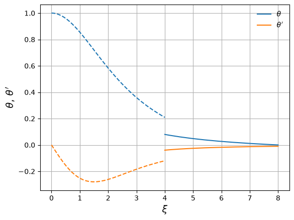
../_images/f823af51303f8d06b7886acff591a710324bdebc2ba9653d47d1016cccd1cbb1.png

We see that there is a large gap in both $θ$ and $θ^{'}$ . This is what our method will try to zero.

Now we rerun until convergence.

n = 3
xi_in, y_in, z_in, xi_out, y_out, z_out = solve_le(n)

corrections:  -0.0010000000, -0.8000000000
corrections:  -0.0011000000,  0.1041147613
corrections:  -0.0012100000, -0.4023120836
corrections:  -0.0013310000,  0.6901802678
corrections:  -0.0014641000, -0.7591982946
corrections:  -0.0016105100,  0.6832784651
corrections:  -0.0017715610, -0.7516063116
corrections:  -0.0019487171,  0.6764456804
corrections:  -0.0021435888, -0.7440902485
corrections:  -0.0023579477,  0.6696812236
corrections:  -0.0025937425, -0.6416966814
corrections:  -0.0028531167,  0.5277816202
corrections:  -0.0031384284, -0.4366105184
corrections:  -0.0034522712,  0.1755129920
corrections:  -0.0037974983, -0.0987626124
corrections:  -0.0006486268,  0.0046186454
corrections:  -0.0000086425, -0.0004880736
corrections:  -0.0000000003,  0.0000000612

fig, ax = plt.subplots()

ax.plot(xi_in, y_in, color="C0", label=r"$\theta$")
ax.plot(xi_out, y_out, color="C0", ls="--")

ax.plot(xi_in, z_in, color="C1", label=r"$\theta'$")
ax.plot(xi_out, z_out, color="C1", ls="--")

ax.set_xlabel(r"$\xi$", fontsize=14)
ax.set_ylabel(r"$\theta,\, \theta'$", fontsize=14)

ax.legend(frameon=False, loc="best")
ax.grid()

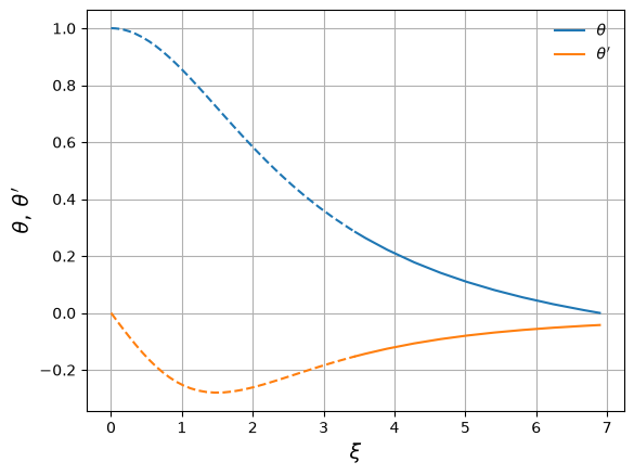
../_images/b0f338ff38e9dba38da2914a0f6fff21a8d78bb92cc4f1a2075696fb08cbf273.png

Now we can get the surface of the polytrope, $ξ_{1}$

xi1 = xi_in[0]
xi1

np.float64(6.896848900808395)

and $θ^{'}$ at the surface:

dthetadxi_1 = z_in[0]

A common quantity needed in finding physical values is $- ξ_{1}^{2} θ^{'} |_{ξ = ξ_{1}}$

-xi1**2 * dthetadxi_1

np.float64(2.0182358018073927)

Application: Stellar Structure

Contents

Application: Stellar Structure#

Polytropes#

Solving the Lane-Emden equation#

Running#