Numerical Errors: Roundoff and Truncation#
We will consider 2 different types of errors:
roundoff error: an error arising from how numbers are represented on computers.
truncation error: an error that arises from approximations we make in turning math operations (like derivatives) into discrete operations that can be done on a computer.
import matplotlib.pyplot as plt
import numpy as np
Roundoff Error#
Computers use finite amount of memory (64-bits for double precision) to store floating point numbers. This means that we cannot represent the infinite set of numbers in the number line in a finite amount of memory. So most numbers are approximate after a certain number of digits.
Exercise
What is (approximately) the smallest number that can be added to 1 such that the result is still distinct from 1
Math is not associative in floating point. Consider
vs
with \(a =\) 1.0, \(b =\) -1.0, and \(c =\) 2.e-15.
Do these two expressions agree?
a = 1.0
b = -1.0
c = 2.e-15

print((a + b) + c)
print(a + (b + c))
2e-15
1.9984014443252818e-15
Reducing roundoff error#
Often we can reduce roundoff error by changing the order of operations or using algebraically equivalent expressions that have better roundoff properties.
For example, subtracting two very large, nearly identical numbers can result in a loss of precision. Consider:
and the equivalent
# the closer together we make these numbers, the larger
# the relative error
a = 1.e18
b = 1.000000001e18

# compute the two algebraically equivalent expressions
f = a**2 - b**2
g = (a - b) * (a + b)

# print both expressions and the relative error
print(f, g, abs((f-g)/g))
-1.9999999769683095e+27 -2.000000001e+27 1.201584528005781e-08
as we make \(a\) and \(b\) closer together, the relative error in the calculation increases.
Exercise
Consider a quadratic equation: \(ax^2 + bx + c\). The two solutions are given by the familiar quadratic equation:
Alternately, we could use the expression:
For values \(a = 0.001\), \(b = 1000\), and \(c = 0.001\), how do we use these expressions to get the most accurate answer?
(example from Newman)
Truncation Error#
Consider Taylor expanding a function \(f(x)\):
Rearranging this, we can solve for \(f^\prime(x)\):
This looks like the definition of a derivative from calculus, but with extra terms that are proportional to \(h\) or higher powers of \(h\).
We can write this as:
where \(\mathcal{O}(h)\) here means that the error in this approximation for the derivative is proportion to \(h\). We say this is first-order accurate. This is an example of truncation error – the terms we are ignoring are an error in our approximation.
Exercise
We can explore the relative importance of roundoff and truncation error.
Consider a first-order approximation to the derivative:
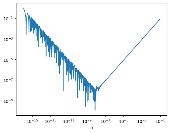
for \(f(x) = \sin(x)\). Plot the error in the approximation, \(D_h(x)\), vs. \(h\). Does it do what you expect?
Let’s discuss the trends:
Starting with the largest value of \(h\), as we make \(h\) smaller, we see that the error decreases. This is following the expected behavior of the truncation error derived above.
Once our \(h\) becomes really small, roundoff error starts to dominate. In effect, we are seeing that:
\[(x_0 + h) - x_0 \ne h\]because of roundoff error.
The minimum error here is around \(\sqrt{\epsilon}\), where \(\epsilon\) is machine epsilon.
Important
Because of roundoff error, we should never exactly compare two floating point numbers, but instead ask that they agree within some tolerance, e.g., test equality as:
Other Errors#
Overflow#
The finite amount of memory used for storing numbers means that there is a maximum and minimum possible number representable as well.

(credit: xkcd)
NaN and Inf#
These are defined “numbers” that represent floating point errors. Consider:
Some NaNs: \(\sqrt{-1}\), \(0/0\), …
Some infs: \(1/0\)
# the largest exponent we can store in double precision
# floating point is 308.  What happens if we go beyond that?
a = 1.e308
print(a*10)
inf


