
Upwinding#
The FTCS discretization was unstable, so let’s try a different discretization. We can approximate the space derivative using a one-sided difference as either:
We’ll choose the one that is an upwinded difference —this means we want to make use of the points from the direction that information is flowing. In our case, \(u > 0\), so we want to use the points to the left of \(i\) in approximating our derivative.
Choosing this difference makes us first-order accurate in space and time. Our difference equation is:
and our update is:
import numpy as np
import matplotlib.pyplot as plt
We’ll use the same grid class as before
class FDGrid:
    """a finite-difference grid"""

    def __init__(self, nx, ng=1, xmin=0.0, xmax=1.0):
        """create a grid with nx points, ng ghost points (on each end)
        that runs from [xmin, xmax]"""

        self.xmin = xmin
        self.xmax = xmax
        self.ng = ng
        self.nx = nx

        # python is zero-based.  Make easy integers to know where the
        # real data lives
        self.ilo = ng
        self.ihi = ng+nx-1

        # physical coords
        self.dx = (xmax - xmin)/(nx-1)
        self.x = xmin + (np.arange(nx+2*ng)-ng)*self.dx

        # storage for the solution
        self.a = self.scratch_array()
        self.ainit = self.scratch_array()

    def scratch_array(self):
        """ return a scratch array dimensioned for our grid """
        return np.zeros((self.nx+2*self.ng), dtype=np.float64)

    def fill_BCs(self):
        """ fill the a single ghostcell with periodic boundary conditions """
        self.a[self.ilo-1] = self.a[self.ihi-1]
        self.a[self.ihi+1] = self.a[self.ilo+1]

    def plot(self):
        fig = plt.figure()
        ax = fig.add_subplot(111)

        ax.plot(self.x[self.ilo:self.ihi+1], self.ainit[self.ilo:self.ihi+1],
                label="initial conditions")
        ax.plot(self.x[self.ilo:self.ihi+1], self.a[self.ilo:self.ihi+1])
        ax.legend()
        return fig
Our upwinding solver is virtually identical to the FTCS solver we just explored.
def upwind_advection(nx, u, C, num_periods=1.0, init_cond=None):
    """solve the linear advection equation using FTCS.  You are required
    to pass in a function f(g), where g is a FDGrid object that sets up
    the initial conditions"""

    g = FDGrid(nx)

    # time info
    dt = C*g.dx/u
    t = 0.0
    tmax = num_periods*(g.xmax - g.xmin)/u

    # initialize the data
    init_cond(g)

    g.ainit[:] = g.a[:]

    # evolution loop
    anew = g.scratch_array()

    while t < tmax:

        if t + dt > tmax:
            dt = tmax - t
            C = u*dt/g.dx

        # fill the boundary conditions
        g.fill_BCs()

        # loop over zones: note since we are periodic and both endpoints
        # are on the computational domain boundary, we don't have to
        # update both g.ilo and g.ihi -- we could set them equal instead.
        # But this is more general
        for i in range(g.ilo, g.ihi+1):
            anew[i] = g.a[i] - C*(g.a[i] - g.a[i-1])

        # store the updated solution
        g.a[:] = anew[:]

        t += dt

    return g
Let’s run it for a period.
def tophat(g):
    g.a[:] = 0.0
    g.a[np.logical_and(g.x >= 1./3, g.x <= 2./3.)] = 1.0
C = 0.5
u = 1.0
nx = 128

g = upwind_advection(nx, u, C, init_cond=tophat)
fig = g.plot()
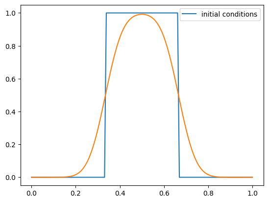
Note
This is stable, but not very accurate. The first-order method is very diffusive.
Smoother initial conditions#
What happens if we start out with smoother initial conditions, like a sine wave?
def sine(g):
    g.a[:] = np.sin(2 * np.pi * g.x)
g = upwind_advection(nx, u, C, init_cond=sine)
fig = g.plot()
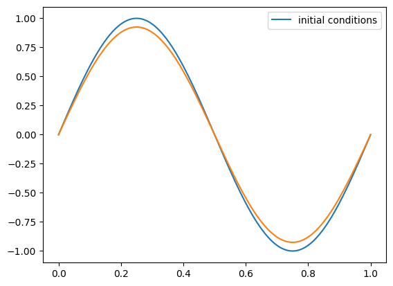
We see that the solution looks better.
Tip
Comparing the solution using our two initial conditions suggests that a lot of the troubles we have are near discontinuities.
Stability#
If we do the same stability truncation analysis as with FTCS, we have:
inserting
and
and grouping terms, we get:
Now we see that the leading error term is \(\mathcal{O}(\Delta x)\), so we are first order accurate, and again, it appears as diffusion, but the diffusion coefficient is positive (physical) so long as:
This is the stability criterion.
C++ implementation#
Here’s a C++ implementation that follows the same ideas as the python version developed here:
fdgrid.H: the grid class#ifndef FDGRID_H #define FDGRID_H #include <iostream> #include <cassert> #include <vector> class Grid { // a finite-difference grid class with nx points and ng ghost points public: int nx; int ng; double xmin; double xmax; int nq; double dx; // indices of the valid domain (i.e. no ghost cells) int ilo; int ihi; // storage for the coordinate std::vector<double> x; // storage for the solution std::vector<double> a; Grid(const int _nx, const int _ng, const double _xmin, const double _xmax) : nx(_nx), ng(_ng), xmin(_xmin), xmax(_xmax), nq(nx + 2*ng), ilo(ng), ihi(ng+nx-1), x(nq, 0.0), a(nq, 0.0) { assert(nx > 0); assert(ng >= 0); assert(xmax > xmin); dx = (xmax - xmin) / static_cast<double>(nx); for (int i = 0; i < nq; ++i) { x[i] = xmin + static_cast<double>(i - ng) * dx; } } void fill_BCs() { // periodic BCs // left edge of domain for (int i = 0; i < ng; ++i) { a[ilo-1-i] = a[ihi-i]; } // right edge of domain for (int i = 0; i < ng; ++i) { a[ihi+1+i] = a[ilo+i]; } } }; #endif
initial_conditions.H: the initial conditions#ifndef INITIAL_CONDITIONS_H #define INITIAL_CONDITIONS_H #include "fdgrid.H" inline void tophat(Grid& g) { // tophat initial conditions for (int i = g.ilo; i <= g.ihi; ++i) { if (g.x[i] > 1.0 / 3.0 && g.x[i] <= 2.0 / 3.0) { g.a[i] = 1.0; } else { g.a[i] = 0.0; } } } #endif
upwind.cpp: the upwind method andmain()#include <iostream> #include <functional> #include <vector> #include "fdgrid.H" #include "initial_conditions.H" Grid upwind(const int nx, const double u, const double C_in, const int num_periods, const std::function<void(Grid&)>& init_cond) { double C = C_in; Grid g(nx, 1, 0.0, 1.0); // time information double dt = C * g.dx / u; double t{0.0}; double tmax = num_periods * (g.xmax - g.xmin) / u; init_cond(g); // evolution loop std::vector<double> a_new(g.nq, 0.0); while (t < tmax) { if (t + dt > tmax) { dt = tmax - t; C = u * dt / g.dx; } // fill boundary conditions g.fill_BCs(); // do upwinding update for (int i = g.ilo; i <= g.ihi; ++i) { a_new[i] = g.a[i] - C * (g.a[i] - g.a[i-1]); } // store the new solution on the grid for (int i = g.ilo; i <= g.ihi; ++i) { g.a[i] = a_new[i]; } t += dt; } return g; } int main() { int nx{64}; double u{1.0}; double C{0.9}; int num_periods{1}; auto g = upwind(nx, u, C, num_periods, tophat); // output for (int i = g.ilo; i <= g.ihi; ++i) { std::cout << g.x[i] << " " << g.a[i] << std::endl; } }
This can be compiled as:
g++ -o upwind upwind.cpp