Example: Lorenz system

Let’s practice writing a solver for an ODE system.

We’ll consider the Lorenz system. This is a toy-model of atmospheric convection. In a seminal paper, Deterministic Nonperiodic Flow, Lorenz explored this system and showed that it exhibited chaotic behavior.

The system can be expressed as:

\[\begin{align*} \frac{dx}{dt} &= \sigma (y - x) \\ \frac{dy}{dt} &= x (r - z) - y \\ \frac{dz}{dt} &= xy - b z \end{align*}\]

where \(x\) is related to the intensity of the convective motion, \(y\) is related to the temperature difference between up and down currents, and \(z\) is related to the departure of the temperature profile from linear (with height). The constants have the following meanings: \(\sigma\) is the Prandtl number, \(r\) is the Rayleigh number (scaled to the critical value), and \(b\) is needed to define the critical Rayleigh number.

Lorenz chose \(\sigma = 10\), \(b = 8/3\), and \(r = 28\)

Exercise

Evolve this system using 4th-order Runge-Kutta and explore how the solution changes with small perturbations to the initial conditions.

sigma = 10.0
b = 8./3.
r = 28.0

import numpy as np
import matplotlib.pyplot as plt

def rhs(xvec):
    x, y, z = xvec
    
    dxdt = sigma * (y - x)
    dydt = x * (r - z) - y
    dzdt = x * y - b * z
    
    return np.array([dxdt, dydt, dzdt])

def integrate(xvec0, dt_in, tmax):
    
    t = 0.0
    dt = dt_in
    
    times = [t]
    history = [np.array(xvec0)]
    
    while t < tmax:
        if t + dt > tmax:
            dt = tmax - t
        
        state_old = history[-1]
        
        k1 = rhs(state_old)
        k2 = rhs(state_old + 0.5 * dt * k1)
        k3 = rhs(state_old + 0.5 * dt * k2)
        k4 = rhs(state_old + dt * k3)
        
        state_new = state_old + (dt / 6.0) * (k1 + 2 * k2 + 2 * k3 + k4)
    
        t += dt
        
        times.append(t)
        history.append(state_new)
        
    return times, history

Let’s run it an look at the solution

xvec0 = np.array([0.0, 0.1, 0.0])

tmax = 40.0
dt = 0.01

times, history = integrate(xvec0, dt, tmax)

xs = [v[0] for v in history]
ys = [v[1] for v in history]
zs = [v[2] for v in history]

fig, ax = plt.subplots()
ax.plot(times, xs, label="x")
ax.plot(times, ys, label="y")
ax.plot(times, zs, label="z")

ax.set_xlabel("t")

ax.legend()

<matplotlib.legend.Legend at 0x7f35941f0790>

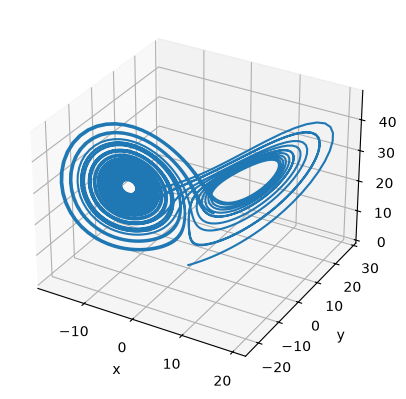
fig = plt.figure()
ax = fig.add_subplot(projection='3d')
ax.plot(xs, ys, zs)
ax.set_xlabel("x")
ax.set_ylabel("y")
ax.set_zlabel("z")

Text(0.5, 0, 'z')

Now let’s run it again with slightly perturbed initial conditions.

xvec0 = np.array([0.0, 0.1001, 0.0])

tmax = 40.0
dt = 0.01

times2, history2 = integrate(xvec0, dt, tmax)

xs2 = [v[0] for v in history2]
ys2 = [v[1] for v in history2]
zs2 = [v[2] for v in history2]

ax.plot(xs2, ys2, zs2)
fig

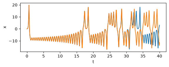
Notice that the solutions track closely for a while and then diverge. We can see this better if we look at just a component.

fig = plt.figure()

ax = fig.add_subplot(211)
ax.plot(times, xs)
ax.plot(times2, xs2)

ax.set_xlabel("t")
ax.set_ylabel("x")

Text(0, 0.5, 'x')