
Application: Recovering Planetary Periods from Radial Velocity Curves#
One method of detecting exoplanets is to look at the motion of a star around the center of mass due to unseen planets–this is the Doppler radial velocity technique.
We’ll look at an idealized example here. Imagine that we have continuous observations of a system and measure the radial velocity of the central star at equally-spaced time-intervals. We can look at the FFT to see what frequencies dominate in the system.
Tip
For real observations, the data points will be unevenly spaced in time, and there will be periods when the system is not observed at all. For this case, the Lomb-Scargle periodogram is a better technique.
import numpy as np
import matplotlib.pyplot as plt
Sample data#
We’ll generate our data using the symplectic integrator / planetary example we explored previously.
Here’s a data file that contains \((t, v_{star,rad})\): radial_velocity.dat
data = np.loadtxt("radial_velocity.dat")
t = data[:, 0]
vel = data[:, 1]
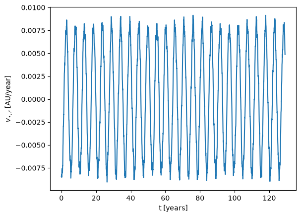
fig, ax = plt.subplots()
ax.plot(t, vel)
ax.set_xlabel("t [years]")
ax.set_ylabel(r"$v_{\star,r}$ [AU/year]")
Text(0, 0.5, '$v_{\\star,r}$ [AU/year]')
Fourier transform#
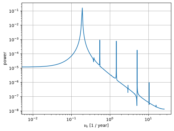
Now we can look at the FFT of the data.
F = np.fft.rfft(vel)
kfreq = np.fft.rfftfreq(len(t), d=t.max() / len(t))
fig, ax = plt.subplots()
ax.plot(kfreq, np.abs(F)**2 * 2 / len(t))
ax.set_xscale("log")
ax.set_yscale("log")
ax.set_ylabel("power")
ax.set_xlabel(r"$\nu_k$ [1 / year]")
ax.grid()
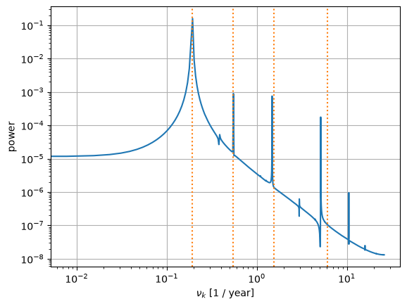
Comparing to truth#
This data was generated with 4 planets around a star with a mass of \(M = 0.3 M_\odot\). In our units, Kepler’s law would be:
The initial semi-major axes were \(a = 2, 1, 0.5, 0.2~\mathrm{AU}\).
So the periods and expected frequencies of the orbits are:
av = np.array([2, 1, 0.5, 0.2])
M = 0.3
Ps = np.sqrt(av**3/M)
freq = 1/Ps
Ps
array([5.16397779, 1.82574186, 0.64549722, 0.16329932])
We can plot these expected frequencies on our FFT.
for f in freq:
    ax.axvline(x=f, color="C1", ls=":")
fig
Plotting the orbits#
We can also look at the data for the planet orbits. Here’s a file that contains the time, and \((x, y)\) positions
of all of the objects (star and planets): planet_positions.dat
data = np.genfromtxt("planet_positions.dat", names=True)
fig, ax = plt.subplots()

ax.plot(data["x_star"], data["y_star"], label="*")
for n in range(1, 5):
    ax.plot(data[f"x_p{n}"], data[f"y_p{n}"], label=f"planet {n}")

ax.set_aspect("equal")
ax.legend()
<matplotlib.legend.Legend at 0x7f3290196900>
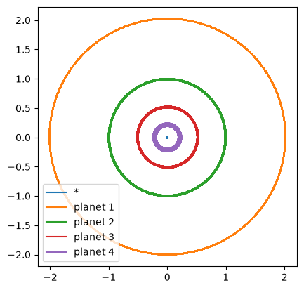
We see that the innermost planet’s orbit is a bit wobbly.