Adaptive RK4 Orbits

We’ll use the same basic ideas in our fixed timestep RK4 integrator.

import numpy as np
import matplotlib.pyplot as plt

# global parameters
GM = 4.0 * np.pi**2  # assuming M = 1 solar mass

OrbitState

The OrbitState class is unchanged.

class OrbitState:
    # a container to hold the star positions
    def __init__(self, x, y, u, v):
        self.x = x
        self.y = y
        self.u = u
        self.v = v

    def __add__(self, other):
        return OrbitState(self.x + other.x, self.y + other.y,
                          self.u + other.u, self.v + other.v)

    def __sub__(self, other):
        return OrbitState(self.x - other.x, self.y - other.y,
                          self.u - other.u, self.v - other.v)

    def __mul__(self, other):
        return OrbitState(other * self.x, other * self.y,
                          other * self.u, other * self.v)

    def __rmul__(self, other):
        return self.__mul__(other)

    def __str__(self):
        return f"{self.x:10.6f} {self.y:10.6f} {self.u:10.6f} {self.v:10.6f}"

Integrator class

We’ll put all of the logical for the integration and stepsize control into a class, called OrbitsRK4. The main Runge-Kutta algorithm that we already explored is now in a function single_step().

class OrbitsRK4:
    """ model the evolution of a single planet around the Sun"""

    def __init__(self, a, e):
        """ a = semi-major axis (in AU),
            e = eccentricity """

        self.a = a
        self.e = e

        x0 = 0.0          # start at x = 0 by definition
        y0 = a*(1.0 - e)  # start at perihelion

        # perihelion velocity (see C&O Eq. 2.33 for ex)
        u0 = -np.sqrt( (GM/a)* (1.0 + e) / (1.0 - e) )
        v0 = 0.0

        self.history = [OrbitState(x0, y0, u0, v0)]
        self.time = [0.0]

        self.n_reset = None

    def kepler_period(self):
        """ return the period of the orbit in yr """
        return np.sqrt(self.a**3)

    def energy(self, n):
        """ return the energy (per unit mass) at time n """

        state = self.history[n]
        return 0.5 * (state.u**2 + state.v**2) - \
            GM / np.sqrt(state.x**2 + state.y**2)

    def rhs(self, state):
        """ RHS of the equations of motion."""

        # current radius
        r = np.sqrt(state.x**2 + state.y**2)

        # position
        xdot = state.u
        ydot = state.v

        # velocity
        udot = -GM * state.x / r**3
        vdot = -GM * state.y / r**3

        return OrbitState(xdot, ydot, udot, vdot)

    def single_step(self, state_old, dt):
        """ take a single RK-4 timestep from t to t+dt for the system
        ydot = rhs """

        # get the RHS at several points
        ydot1 = self.rhs(state_old)

        state_tmp = state_old + 0.5 * dt * ydot1
        ydot2 = self.rhs(state_tmp)

        state_tmp = state_old + 0.5 * dt * ydot2
        ydot3 = self.rhs(state_tmp)

        state_tmp = state_old + dt * ydot3
        ydot4 = self.rhs(state_tmp)

        # advance
        state_new = state_old + (dt / 6.0) * (ydot1 + 2.0 * ydot2 +
                                              2.0 * ydot3 + ydot4)

        return state_new

    def integrate(self, dt_in, err, tmax):
        """ integrate the equations of motion using 4th order R-K method with an
            adaptive stepsize, to try to achieve the relative error err.  dt
            here is the initial timestep
            """
        
        # start with the old timestep
        dt_new = dt_in
        dt = dt_in

        n_reset = 0
        t = 0

        while t < tmax:
            
            state_old = self.history[-1]

            if err > 0.0:

                # adaptive stepping iteration loop -- keep trying to take a step
                # until we achieve our desired error

                rel_error = 1.e10

                n_try = 0
                while rel_error > err:
                    dt = min(dt_new, tmax-t)

                    # take 2 half steps
                    state_tmp = self.single_step(state_old, 0.5*dt)
                    state_new = self.single_step(state_tmp, 0.5*dt)

                    # now take just a single step to cover dt
                    state_single = self.single_step(state_old, dt)

                    # state_new should be more accurate than state_single since it
                    # used smaller steps

                    # estimate the relative error now
                    dstate = state_new - state_single

                    rel_error = max(abs(dstate.x / state_single.x),
                                    abs(dstate.y / state_single.y),
                                    abs(dstate.u / state_single.u),
                                    abs(dstate.v / state_single.v))

                    # adaptive timestep algorithm for RK4

                    dt_est = dt * abs(err/rel_error)**0.2

                    # give a little safety in our dt_est, and limit the
                    # amount the timestep can change 
                    dt_new = min(max(0.9 * dt_est, 0.25 * dt), 4.0 * dt)

                    n_try += 1

                if n_try > 1:
                    # n_try = 1 if we took only a single try at the step
                    n_reset += (n_try-1)

            else:

                # take just a single step
                dt = min(dt_new, tmax-t)

                # take just a single step to cover dt
                state_new = self.single_step(state_old, dt)

            # successful step
            t += dt

            # store
            self.time.append(t)
            self.history.append(state_new)

        self.n_reset = n_reset

    def plot(self, points=False):
        """plot the orbit"""
        fig, ax = plt.subplots()
        x = [q.x for q in self.history]
        y = [q.y for q in self.history]

        # draw the Sun
        ax.scatter([0], [0], marker=(20, 1), color="y", s=250)

        if points:
            ax.scatter(x, y, marker=".")
        else:
            ax.plot(x, y)
        ax.set_aspect("equal")
        return fig

Note

We have a lot of freedom in how we define our error. We could use an absolute error instead of a relative error, we could also only consider certain components (like \(x\) and \(y\)), etc.

Highly eccentric orbit

Let’s create an orbit with a tolerance of \(10^{-5}\), and the a very high eccentricity (\(a = 1\), \(e = 0.95\))

o = OrbitsRK4(1.0, 0.95)
o.integrate(0.05, 1.e-5, o.kepler_period())

How many points did it take?

len(o.history)

92

and how many times did we reset?

o.n_reset

39

Let’s plot it

fig = o.plot(points=True)
fig.set_size_inches(5, 12)

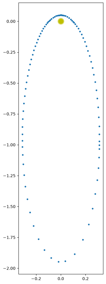
Clearly we see that the size of the timestep is much larger at aphelion as compared to perihelion.

Let’s create a version with a fixed timestep, with a timestep of \(0.001~\mathrm{yr}\). We can do this by passing in a negative error.

o_fixed = OrbitsRK4(1.0, 0.95)
o_fixed.integrate(0.001, -1, o_fixed.kepler_period())
fig = o_fixed.plot()
fig.set_size_inches(5, 12)

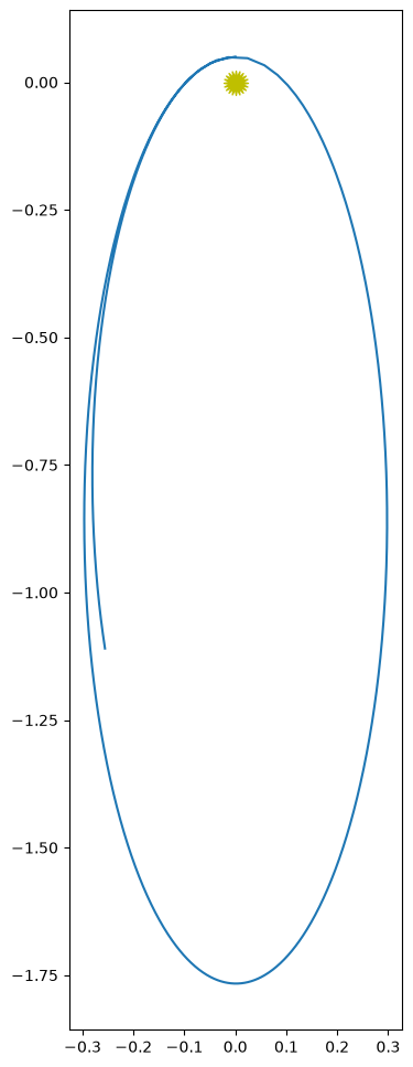
len(o_fixed.history)

1001

We need a really small fixed step size to integrate this at all reasonably

Timestep evolution

Let’s look at the adaptive version some more. First, let’s look at the timestep evolution.

ts = np.array(o.time)

dt = ts[1:] - ts[:-1]
tc = 0.5 * (ts[1:] + ts[:-1])

fig, ax = plt.subplots()
ax.plot(tc, dt)
ax.set_xlabel("t [yr]")
ax.set_ylabel("dt [yr]")
ax.set_yscale("log")

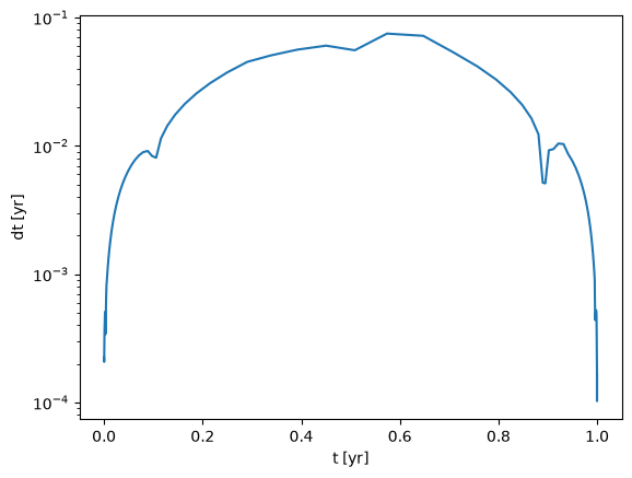
Notice that the timestep changes by ~ 3 orders of magnitude over the evolution.

Energy conservation

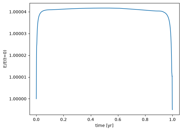
What about energy conservation?

e = []
ts = o.time
for n in range(len(o.history)):
    e.append(o.energy(n))
    
fig, ax = plt.subplots()
ax.plot(ts, e/e[0])
ax.set_xlabel("time [yr]")
ax.set_ylabel("E/E(t=0)")
ax.ticklabel_format(useOffset=False)

Now let’s do 10 orbits

o = OrbitsRK4(1.0, 0.95)
o.integrate(0.05, 1.e-5, 20*o.kepler_period())

e = []
ts = o.time
for n in range(len(o.history)):
    e.append(o.energy(n))
    
fig, ax = plt.subplots()
ax.plot(ts, e/e[0])
ax.set_xlabel("time [yr]")
ax.set_ylabel("E/E(t=0)")
ax.ticklabel_format(useOffset=False)

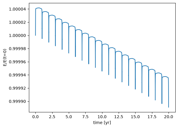
Caution

We can see that RK4 does not conserve energy!

There is a steady decrease in the total energy over 20 orbits. If we wanted to evolve for millions of years, this would certainly be a problem. Making the tolerance tighter certainly will help, but it will also make things a lot more expensive.

The problem is that 4th order Runge-Kutta does not know anything about energy conservation.

C++ implementation

A C++ implementation following the same ideas is available as orbit_adaptive.cpp

#include <iostream>
#include <vector>
#include <iomanip>
#include <cmath>
#include <numeric>
#include <limits>
#include <fstream>

const double GM = 4.0 * M_PI * M_PI;

struct OrbitState {
    // a container to hold the star positions
    double x{};
    double y{};
    double u{};
    double v{};

    OrbitState(double x0, double y0, double u0, double v0)
        : x{x0}, y{y0}, u{u0}, v{v0}
    {}

    OrbitState() {}

    OrbitState operator+(const OrbitState& other) const {
        return OrbitState(x + other.x, y + other.y, u + other.u, v + other.v);
    }

    OrbitState operator-(const OrbitState& other) const {
        return OrbitState(x - other.x, y - other.y, u - other.u, v - other.v);
    }

    OrbitState operator*(double a) const {
        return OrbitState(a * x, a * y, a * u, a * v);
    }

};

std::ostream& operator<< (std::ostream& os, const OrbitState& s) {
    os.precision(6);

    os << std::setw(14) << s.x
       << std::setw(14) << s.y
       << std::setw(14) << s.u
       << std::setw(14) << s.v;

    return os;
}

inline
OrbitState operator*(double a, const OrbitState& state) {
    return OrbitState(a * state.x, a * state.y, a * state.u, a * state.v);
}

class OrbitsRK4 {
    // model the evolution of a single planet around the Sun using gravitational
    // interaction of three stars

private:

    // a vector to store the history of our orbit
    std::vector<OrbitState> history;
    std::vector<double> time;
    int n_reset{0};

public:

    OrbitsRK4(const double a, const double e)  {

        OrbitState initial_conditions;

        // put the planet at perihelion

        initial_conditions.x = 0.0;
        initial_conditions.y = a * (1.0 - e);
        initial_conditions.u = std::sqrt((GM / a) * (1.0 + e) / (1.0 - e));
        initial_conditions.v = 0.0;

        history.push_back(initial_conditions);

        time.push_back(0.0);
    }

    int npts() {
        // return the number of integration points
        return time.size();
    }

    int get_n_reset() {
        // return the number of times a step was reset
        return n_reset;
    }

    double get_time(const int n) {
        // return the physical time for step n
        return time[n];
    }

    OrbitState& get_state(const int n) {
        // return a reference to the state at time index n
        return history[n];
    }

    double energy(const int n) {
        // return the energy of the system for timestep n

        const auto& state = history[n];

        // kinetic energy

        double KE = 0.5 * (state.u * state.u + state.v * state.v);
        double PE = -GM / std::sqrt(state.x * state.x + state.y * state.y);
        return KE + PE;
    }

    OrbitState rhs(const OrbitState& state) {
        // compute the ydot terms

        OrbitState ydot;

        ydot.x = state.u;
        ydot.y = state.v;

        double dx = state.x;
        double dy = state.y;

        double r = std::sqrt(dx * dx + dy * dy);

        ydot.u = -GM * dx / std::pow(r, 3);
        ydot.v = -GM * dy / std::pow(r, 3);

        return ydot;

    }

    OrbitState single_step(const OrbitState& state_old, const double dt) {
        /// take a single RK-4 timestep through dt

        auto ydot1 = rhs(state_old);

        OrbitState state_temp;

        state_temp = state_old + 0.5 * dt * ydot1;
        auto ydot2 = rhs(state_temp);

        state_temp = state_old + 0.5 * dt * ydot2;
        auto ydot3 = rhs(state_temp);

        state_temp = state_old + dt * ydot3;
        auto ydot4 = rhs(state_temp);

        OrbitState s = state_old + (dt / 6.0) *
            (ydot1 + 2.0 * ydot2 + 2.0 * ydot3 + ydot4);

        return s;
    }


    void integrate(const double dt_in, const double err, const double tmax) {
        // integrate the equations of motion using 4th order R-K
        // method with an adaptive stepsize, to try to achieve the
        // relative error err.  dt here is the initial timestep

        // if err < 0, then we don't do adaptive stepping, but rather
        // we always walk at the input dt

        // start with the old timestep
        double dt_new{dt_in};
        double dt{dt_in};

        double t{0.0};

        while (t < tmax) {

            const auto &state_old = history.back();

            // adaptive stepping iteration loop -- keep trying to take
            // a step until we achieve our desired error
            double rel_error = std::numeric_limits<double>::max();

            int n_try{0};

            OrbitState state_new;

            while (rel_error > err) {

                dt = std::min(dt_new, tmax - t);

                // take 2 half steps

                auto state_temp = single_step(state_old, 0.5*dt);
                state_new = single_step(state_temp, 0.5*dt);

                // now take just a single step to cover dt

                auto state_single = single_step(state_old, dt);

                // state_new should be more accurate than state_single
                // since it used smaller steps

                // estimate the relative error now

                double pos_err =
                    std::max(std::abs((state_new.x - state_single.x) /
                                      state_single.x),
                             std::abs((state_new.y - state_single.y) /
                                      state_single.y));

                double vel_err =
                    std::max(std::abs((state_new.u - state_single.u) /
                                      state_single.u),
                             std::abs((state_new.v - state_single.v) /
                                      state_single.v));

                rel_error = std::max(pos_err, vel_err);

                // adaptive timestep algorithm from Garcia (Eqs. 3.30
                // and 3.31)

                double dt_est = dt * std::pow(std::abs(err/rel_error), 0.2);
                dt_new = std::min(std::max(0.9 * dt_est, 0.25 * dt), 4.0 * dt);

                n_try++;
            }

            if (n_try > 1) {
                // n_try = 1 if we took only a single try at the step
                n_reset += (n_try - 1);
            }

            // successful step
            t += dt;

            // store the new solution -- this will automatically be
            // used as the "old" state in the next step

            time.push_back(t);
            history.push_back(state_new);

        }

    }
};


int main() {

    OrbitsRK4 o(1.0, 0.95);
    o.integrate(0.05, 1.e-5, 1.0);

    std::cout << "number of points = " << o.npts() << std::endl;
    std::cout << "number of times a step was rejected = "
              << o.get_n_reset() << std::endl;

    std::ofstream of("orbit_adaptive.dat");

    for (int n = 0; n < o.npts(); ++n) {
        const auto& state = o.get_state(n);

        of << std::setw(14) << o.get_time(n);

        of << state;

        of.precision(10);

        of << std::setw(18) << o.energy(n);

        of << std::endl;

    }

}