Composite Integration

It usually doesn’t pay to go to higher-order polynomials (e.g., fitting a cubic to 4 points in the domain). Instead, we can do composite integration by dividing our domain \([a, b]\) into slabs, and then using the above approximations.

Here’s an illustration of dividing the domain into 6 slabs:

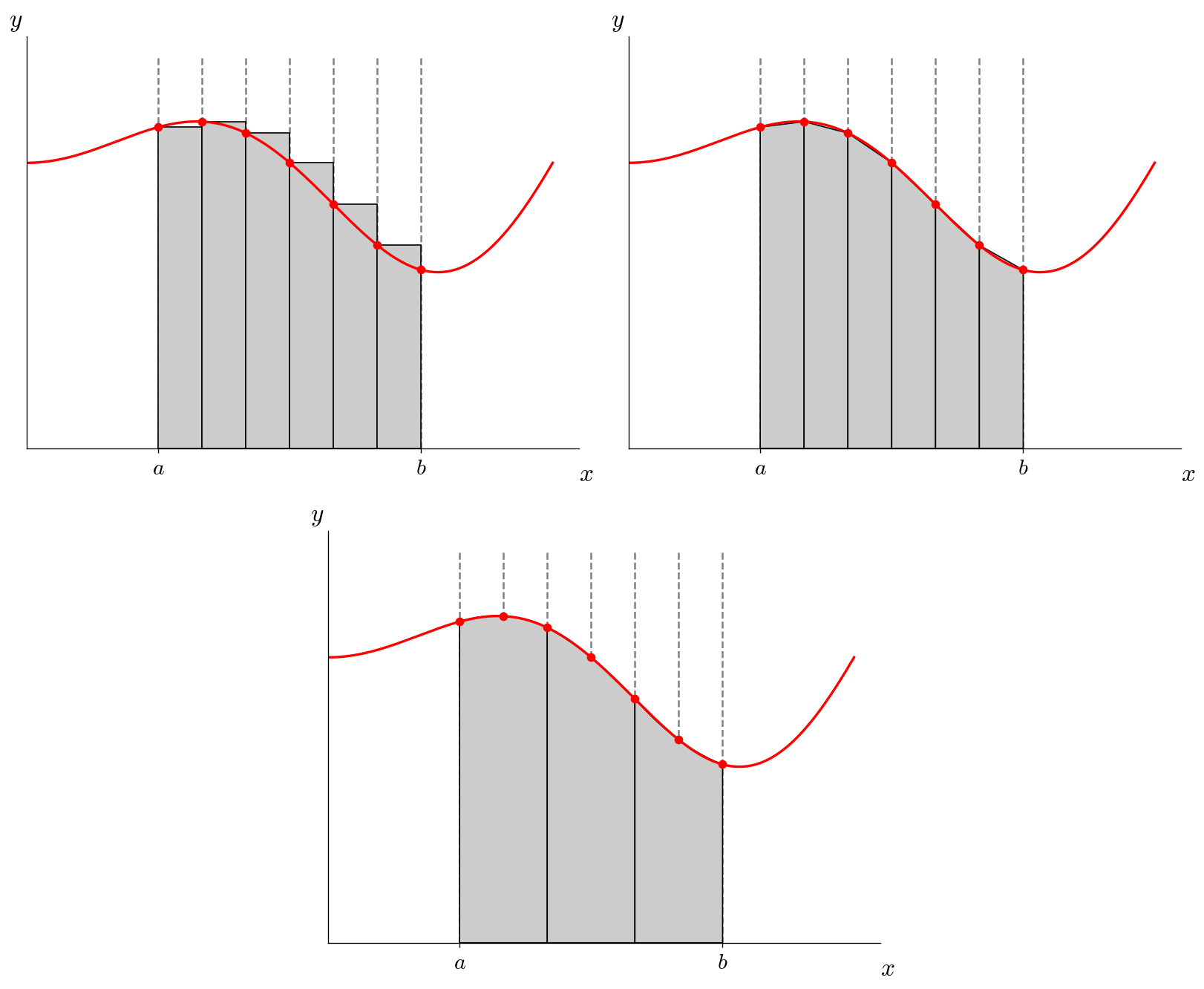
Imagine using \(N\) slabs. For the rectangle and trapezoid rules, we would apply them N times (once per slab) and sum up the integrals in each slab. For the Simpson’s rule, we would apply Simpson’s rule over 2 slabs at a time and sum up the integrals over the \(N/2\) pair of slabs (this assumes that \(N\) is even).

The composite rule for trapezoid integration is:

\[ \int_a^b f(x) dx = \frac{\Delta x}{2} \sum_{i=0}^{N-1} (f_i + f_{i+1}) + \mathcal{O}(\Delta x^2) \]

and for Simpson’s rule, it is:

\[ \int_a^b f(x) dx = \frac{\Delta x}{3} \sum_{i = 0}^{N/2-1} (f_{2i} + 4 f_{2i+1} + f_{2i+2}) + \mathcal{O}(\Delta x^4) \]

Example

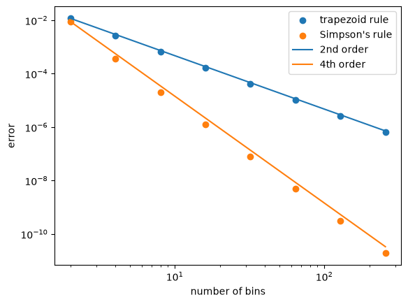
For the function in the previous exercise, perform a composite integral using the trapezoid and Simpson’s rule for \(N = 2, 4, 8, 16, 32\). Compute the error with respect to the analytic solution and make a plot of the error vs. \(N\) for both methods. Do the errors follow the scaling shown in the expressions above?

import numpy as np
import matplotlib.pyplot as plt

First let’s write the function we will integrate

def f(x):
    return 1 + 0.25 * x * np.sin(np.pi * x)

Now our composite trapezoid and Simpson’s rules. These functions will take the number of bins, \(N\), and the integration limits \([a, b]\) and then sample our function at \(N+1\) points to do the composite integration.

def I_t(N, a, b, func):
    """composite trapezoid rule.  Here N is the number
    of bins, [a, b] are the integration limits, and
    func is the function to call."""
    
    I = 0.0
    x = np.linspace(a, b, N+1)
    
    # loop over bins
    for n in range(N):
        I += 0.5*(x[n+1] - x[n]) * (func(x[n]) + func(x[n+1]))
    return I

def I_s(N, a, b, func):
    """composite Simpsons rule.  Here N is the number
    of bins, [a, b] are the integration limits, and
    func is the function to call."""
    
    # we require an even number of bins
    assert N % 2 == 0
    
    I = 0.0
    x = np.linspace(a, b, N+1)
    
    # loop over bins
    for n in range(0, N-1, 2):
        dx = x[n+1] - x[n]
        I += dx/3.0 * (f(x[n])+ 4 * f(x[n+1]) + f(x[n+2]))
    return I

Integration limits

a = 0.5
b = 1.5

The analytic solution

I_a = 1 - 1/(2 * np.pi**2)

Now let’s run for a bunch of different number of bins and store the errors

# number of bins
N = [2, 4, 8, 16, 32, 64, 128, 256]

# keep track of the errors for each N
err_trap = []
err_simps = []

for nbins in N:
    err_trap.append(np.abs(I_t(nbins, a, b, f) - I_a))
    err_simps.append(np.abs(I_s(nbins, a, b, f) - I_a))

Now we’ll plot the errors along with the expected scaling

err_trap = np.asarray(err_trap)
err_simps = np.asarray(err_simps)
N = np.asarray(N)

fig = plt.figure()
ax = fig.add_subplot(111)

ax.scatter(N, err_trap, label="trapezoid rule")
ax.scatter(N, err_simps, label="Simpson's rule")

# compute the ideal scaling
# err = err_0 (N_0 / N) ** order
fourth_order = err_simps[0] * (N[0]/N)**4
second_order = err_trap[0] * (N[0]/N)**2

ax.plot(N, second_order, label="2nd order")
ax.plot(N, fourth_order, label="4th order")

ax.set_xscale("log")
ax.set_yscale("log")

ax.legend()
ax.set_xlabel("number of bins")
ax.set_ylabel("error")

Text(0, 0.5, 'error')

Warning

As you make the number of bins larger and larger, eventually you’ll hit a limit to how accurate you can get the integral (somewhere around N ~ 4096 bins for Simpson’s). Beyond that, roundoff error dominates.

C++ implementation

Here’s a C++ implementation: simpsons.cpp

#include <iostream>
#include <iomanip>
#include <cmath>
#include <functional>
#include <cassert>
#include <numbers>

// An implementation of the composite Simpsons rule for integration.  This
// assumes that we will use an even number of intervals

// note: requires C++20 due to std::numbers

// the function we will integrate
double f(const double x) {
    return 1.0 + x * std::sin(std::numbers::pi * x) / 4.0;
}

// the analytic integral of f(x) over [1/2, 3/2]
double I_analytic() {
    return 1.0 - 0.5 / std::pow(std::numbers::pi, 2);
}

// implement the composite simpsons rule.  Here N is the number
// of intervals, so there will be N+1 points from xmin to xmax
double simpsons(const double xmin, const double xmax, const int N,
                std::function<double(const double)> func) {

    assert(N % 2 == 0);

    double I = 0.0;
    double dx = (xmax - xmin) / static_cast<double>(N);

    for (int n = 0; n < N; n += 2) {
        double x0 = xmin + static_cast<double>(n) * dx;
        I += dx / 3.0 * (func(x0) + 4.0 * func(x0 + dx) + func(x0 + 2.0*dx));
    }

    return I;
}

int main() {

    double xmin{0.5};
    double xmax{1.5};

    for (auto N : {2, 4, 8, 16, 32, 64}) {
        double I = simpsons(xmin, xmax, N, f);
        double err = std::abs(I - I_analytic());
        std::cout << std::setw(3) << N << ": " << err << std::endl;
    }
}