Linear Interpolation

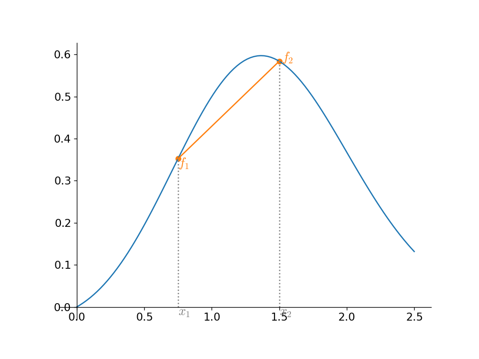
The simplest interpolation we can imagine is doing connect-the-dots, and simply connecting our data samples with straight lines.

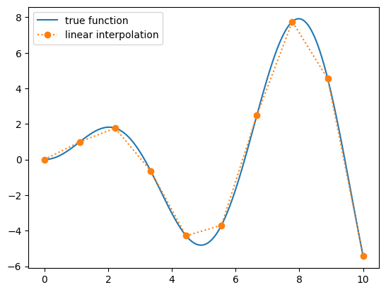
As we see, this only gets the correct values at the end points (for a general function), but it has the nice property that it does not introduce any new minima or maxima.

Given some N points sampling a function, \((x_i, f_i)\), the interpolant connecting the points \(i\) and \(i+1\) is:

\[f(x) = \frac{f_{i+1} - f_i}{x_{i+1} - x_i} (x - x_i) + f_i\]

for \(x_i \le x \le x_{i+1}\)

For N points, we have \(N-1\) interpolants.

Piecewise interpolation

This is an example of piecewise interpolation. We don’t try to fit all of the points with a single polynomial, but instead fit a subset of points with a low-order polynomial (in this case, a line).

Example

Let’s write a function to tabulate \(f(x) = x \sin(x)\) on \([0, 5]\) and then use linear interpolation to get the function values.

How many function samples do we need to get a 1% error?

import numpy as np
import matplotlib.pyplot as plt

def f(x):
    return x * np.sin(x)

def sample_function(func, npts, *, xmin=0.0, xmax=10.0):
    xx = np.linspace(xmin, xmax, npts)
    return xx, func(xx)

Let’s look at this function and 10 samples

fig, ax = plt.subplots()
xmin = 0.0
xmax = 10.0
N = 10

x_fine = np.linspace(xmin, xmax, 1000)
x_sample, f_sample = sample_function(f, N, xmin=xmin, xmax=xmax)

ax.plot(x_fine, f(x_fine), label="true function")
ax.plot(x_sample, f_sample, marker="o", ls=":", label="linear interpolation")
ax.legend()

<matplotlib.legend.Legend at 0x7f1d95fb77d0>

Now let’s define our interpolate function. This will take the location and values where the function is sampled, (xv, fv), and the location where we want to approximate the value of the underlying function, x0.

def interpolate(x0, xv, fv):
    
    # find first x[i] > x0
    idx = np.argwhere(xv > x0)[0][0]
    
    # we want to use this point and the one to the left
    # we'll shift idx to point to the left point
    idx = max(0, idx-1)
    
    slope = (fv[idx+1] - fv[idx]) / (xv[idx+1] - xv[idx])
    return slope * (x0 - xv[idx]) + fv[idx]

Let’s just look at \(x_0 = 4.5\) (this is near a minimum) and try different number of points and measure the error

x0 = 4.5

for n in [5, 10, 20, 40, 80, 160]:
    xv, fv = sample_function(f, n)

    finterp = interpolate(x0, xv, fv)
    fexact = f(x0)
    err = np.abs(finterp - fexact)
    print(f"{n:4} points, error = {err}")

   5 points, error = 0.8624245028923605
  10 points, error = 0.14257394829953363
  20 points, error = 0.1333081368280027
  40 points, error = 0.03204962648664189
  80 points, error = 0.007851522573614211
 160 points, error = 0.0019427475977087383

In this case, after 80 points, our error is < 1%.

We also see that we appear to converge slightly better than 2nd order

C++ implementation

Here’s a C++ version that follows the same ideas:

#include <iostream>
#include <cmath>
#include <vector>
#include <functional>
#include <print>

// our test function

double f(double x) {
    return x * std::sin(x);
}


// a function that will produce N samples of the input func(x)

std::pair<std::vector<double>, std::vector<double>>
sample_function(std::function<double(double)> func,
                int npts, double xmin, double xmax) {

    std::vector<double> xv(npts, 0.0);
    std::vector<double> fv(npts, 0.0);

    double dx = (xmax - xmin) / static_cast<double>(npts - 1);

    for (int i = 0; i < npts; ++i) {
        xv[i] = xmin + static_cast<double>(i) * dx;
        fv[i] = func(xv[i]);
    }

    return {xv, fv};
}


// the main linear intepolation function

double interpolate(double x0,
                   const std::vector<double>& xv,
                   const std::vector<double>& fv) {

    // find the index i where xv[i] > x0
    int idx = -1;
    for (std::size_t i = 0; i < xv.size()-1; ++i) {
        if (x0 > xv[i] && x0 < xv[i+1]) {
            idx = i;
            break;
        }
    }

    if (idx == -1) {
        std::cout << "x0 is not in range of xv" << std::endl;
    }

    double slope = (fv[idx+1] - fv[idx]) / (xv[idx+1] - xv[idx]);
    return slope * (x0 - xv[idx]) + fv[idx];
}


// test driver

int main() {

    // we want to find the N such that the error in our interpolation
    // is < 1%.  We'll just consider a bunch of different sizes for N

    double xmin{0.0};
    double xmax{10.0};
    double x0{4.5};

    for (auto N : {5, 10, 20, 40, 80, 160}) {
        const auto [xv, fv] = sample_function(f, N, xmin, xmax);

        auto finterp = interpolate(x0, xv, fv);
        auto fexact = f(x0);

        double err = std::abs(finterp - fexact);

        std::println("{:4} points, error = {:7.5f}", N, err);
    }
}