
Testing Our Least Squares#
We’ll write a general linear least squares implementation and test it first on a parabolic fit and then on a higher-order polynomial.
Parabolic fit#
Let’s consider fitting to a function:
for \(M = 3\), this is:
If we have 10 data points, \(x_1, \ldots, x_{10}\), then our matrix \({\bf A}\) will take the form:
import numpy as np
import matplotlib.pyplot as plt
Let’s first write a function that takes an \(x_i\) and returns the entries in a row of \({\bf A}\)
def basis(x, M=3):
    """ the basis function for the fit, x**n"""

    j = np.arange(M)
    return x**j
Now we’ll write a function that takes our data and errors and sets up the linear system \({\bf A}^\intercal {\bf A} {\bf a} = {\bf A}^\intercal {\bf b}\) and solves it.
def general_regression(x, y, yerr, M):
    """ here, M is the number of fitting parameters.  We will fit to
        a function that is linear in the a's, using the basis functions
        x**j """

    N = len(x)

    # construct the design matrix -- A_{ij} = Y_j(x_i)/sigma_i -- this is
    # N x M.  Each row corresponds to a single data point, x_i, y_i
    A = np.zeros((N, M), dtype=np.float64)

    for i in range(N):
        A[i,:] = basis(x[i], M) / yerr[i]

    # construct the MxM matrix for the linear system, A^T A:
    ATA = np.transpose(A) @ A

    print("condition number of A^T A:", np.linalg.cond(ATA))

    # construct the RHS
    b = np.transpose(A) @ (y / yerr)

    # solve the system
    a = np.linalg.solve(ATA, b)

    # return the chisq
    chisq = 0
    for i in range(N):
        chisq += (np.sum(a*basis(x[i], M)) - y[i])**2 / yerr[i]**2

    chisq /= N-M

    return a, chisq
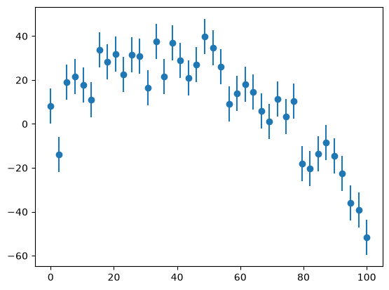
Finally, we’ll make up some experiment data that follows a parabola, but with a perturbation.
def y_experiment2(a1, a2, a3, sigma, x):
    """ return the experimental data and error in a quadratic +
    random fashion, with a1, a2, a3 the coefficients of the
    quadratic and sigma is scale of the error.  This will be
    poorly matched to a linear fit for a3 != 0 """

    N = len(x)

    # this creates a Gaussian normal random number from a distribution
    # centered on 0 with a width of sigma
    rng = np.random.default_rng()
    r = sigma * rng.standard_normal(N)

    y = a1 + a2*x + a3*x*x + r

    return y, np.ones_like(y) * sigma
N = 40
x = np.linspace(0, 100.0, N)

# one-sigma error
sigma = 8.0

y, yerr = y_experiment2(2.0, 1.50, -0.02, sigma, x)
fig, ax = plt.subplots()

ax.errorbar(x, y, yerr=yerr, fmt="o")
<ErrorbarContainer object of 3 artists>
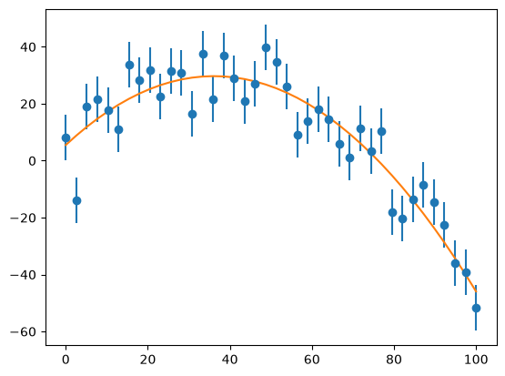
Now let’s do the fit of a parabola. Along the way, we’ll print out the condition number of the matrix \({\bf A}^\intercal{\bf A}\).
# do the regression with M = 3 (1, x, x^2)
M = 3
a, chisq = general_regression(x, y, yerr, M)
condition number of A^T A: 169717921.7386773
Notice that the condition number is quite large!
ax.plot(x, a[0] + a[1]*x + a[2]*x*x)
fig
Higher order fit#
fig, ax = plt.subplots()
M = 10
a, chisq = general_regression(x, y, yerr, M)
yfit = np.zeros((len(x)), dtype=x.dtype)
for i in range(N):
    base = basis(x[i], M)
    yfit[i] = np.sum(a*base)

ax.errorbar(x, y, yerr=yerr, fmt="o")
ax.plot(x, yfit)
condition number of A^T A: 1.8806097126766699e+34
[<matplotlib.lines.Line2D at 0x7f8c56d30d70>]
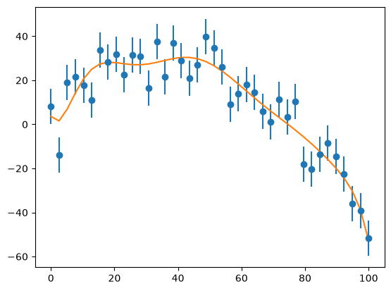
The \(M = 10\) polynomial fits, but the condition number is large. It is not clear that going higher order here is wise.
Fitting and condition number#
It can be shown that if your basis function is orthonormal in the interval you are fitting over, then the condition number of the matrix \({\bf A}^\intercal {\bf A}\) will be much lower. For example, it we fit to the interval \([-1, 1]\), then the Legendre polynomials are a good basis.
The text by Yakowitz & Szidarovszky has a good discussion on this.
Errors in the fitting parameters#
It can also be shown that the errors in the fitting parameters are:
where
is the covariance matrix.
C++ implementation#
For the C++ implementation, we create a Matrix class, contained in matrix.H, that overloads * to do
matrix-matrix and matrix-vector multiplication.
We also reuse our Gaussian elimination code from before.
matrix.H: the `Matrix class#ifndef MATRIX_H #define MATRIX_H #include <vector> #include <iostream> #include <iomanip> #include <cassert> // a 2-d matrix with contiguous storage // here the data is stored in row-major order in a 1-d memory space // managed as a vector. We overload () to allow us to index this as // a(irow, icol) struct Matrix { std::size_t _rows; std::size_t _cols; std::vector<double> _data; Matrix (std::size_t rows, std::size_t cols, double val=0.0) : _rows{rows}, _cols{cols}, _data(rows * cols, val) { assert (rows > 0 && cols > 0); } // Constructor for list initialization // e.g., Matrix A{{1, 2}, {3, 4}}; Matrix(std::initializer_list<std::initializer_list<double>> values) : _rows(values.size()), _cols(values.begin()->size()), _data() { assert(_rows > 0); for (const auto& row : values) { // Ensure all rows have the same number of columns assert(row.size() == _cols); _data.insert(_data.end(), row.begin(), row.end()); } } // note the "const" after the argument list here -- this means // that this can be called on a const Matrix [[nodiscard]] inline std::size_t ncols() const { return _cols;} [[nodiscard]] inline std::size_t nrows() const { return _rows;} inline double& operator()(std::size_t row, std::size_t col) { // size_t is unsigned, so will always be >= 0 assert (row < _rows); assert (col < _cols); return _data[row*_cols + col]; } inline const double& operator()(std::size_t row, std::size_t col) const { // size_t is unsigned, so will always be >= 0 assert (row < _rows); assert (col < _cols); return _data[row*_cols + col]; } Matrix transpose() { Matrix A_T(_cols, _rows); for (std::size_t irow = 0; irow < _rows; ++irow) { for (std::size_t jcol = 0; jcol < _cols; ++jcol) { A_T(jcol, irow) = (*this)(irow, jcol); } } return A_T; } std::vector<double> operator* (const std::vector<double>& x) { // do b = A x assert (_cols == x.size()); std::vector<double> b(_rows, 0.0); for (std::size_t irow = 0; irow < _rows; ++irow) { for (std::size_t k = 0; k < _cols; ++k) { b[irow] += (*this)(irow, k) * x[k]; } } return b; } Matrix operator* (const Matrix& B) { // do C = A B assert (_cols == B.nrows()); Matrix C(_rows, B.ncols()); for (std::size_t irow = 0; irow < C.nrows(); ++irow) { for (std::size_t jcol = 0; jcol < C.ncols(); ++jcol) { for (std::size_t k = 0; k < _cols; ++k) { C(irow, jcol) += (*this)(irow, k) * B(k, jcol); } } } return C; } }; // the << operator is not part of the of the class, so it is not a // member inline std::ostream& operator<< (std::ostream& os, const Matrix& a) { std::cout << std::setprecision(4) << std::fixed; for (std::size_t row = 0; row < a.nrows(); ++row) { for (std::size_t col = 0; col < a.ncols(); ++col) { os << std::setw(8) << a(row, col) << " "; } os << std::endl; } return os; } #endif
gauss.H: the Gaussian elimination function#ifndef GAUSS_H #define GAUSS_H #include <algorithm> #include <vector> #include <limits> #include <iostream> #include <iomanip> #include "matrix.H" inline std::vector<double> gauss_elim(Matrix& A, std::vector<double>& b) { // perform gaussian elimination with pivoting, solving A x = b. // // A is an NxN matrix, x and b are an N-element vectors. Note: A and b are // changed upon exit to be in upper triangular (row echelon) form auto N = b.size(); // A is square, with each dimension of length N assert(A.nrows() == N && A.ncols() == N); // allocate the solution array std::vector<double> x(N, 0.0); // main loop over rows for (std::size_t krow = 0; krow < N; ++krow) { // find the pivot row based on the size of column k -- only // consider the rows beyond the current row auto row_max{krow}; double col_max = std::numeric_limits<double>::lowest(); for (std::size_t kk = krow; kk < N; ++kk) { if (std::abs(A(kk, krow)) > col_max) { col_max = std::abs(A(kk, krow)); row_max = kk; } } // swap the row with the largest element in the current column // with the current row (pivot) -- do this with b too! if (row_max != krow) { for (std::size_t jcol = 0; jcol < N; ++jcol) { std::swap(A(krow, jcol), A(row_max, jcol)); } std::swap(b[krow], b[row_max]); } // do the forward-elimination for all rows below the current for (std::size_t irow = krow+1; irow < N; ++irow) { double coeff = A(irow, krow) / A(krow, krow); for (std::size_t jcol = krow+1; jcol < N; ++jcol) { A(irow, jcol) += -A(krow, jcol) * coeff; } A(irow, krow) = 0.0; b[irow] += -coeff * b[krow]; } } // back-substitution x[N-1] = b[N-1] / A(N-1, N-1); // size_t is unsigned, so it is never < 0, it will // wrap to a large number for (std::size_t irow = N-2; irow != std::numeric_limits<std::size_t>::max(); --irow) { std::cout << irow << std::endl; double bsum = b[irow]; for (std::size_t jcol = irow+1; jcol < N; ++jcol) { bsum += -A(irow, jcol) * x[jcol]; } x[irow] = bsum / A(irow, irow); } return x; } #endif
fitting.H: the generalized least squares fitting function#include <cassert> #include <cmath> #include <iostream> #include <vector> #include "matrix.H" #include "gauss.H" std::pair<std::vector<double>, double> general_regression(const std::vector<double>& x, const std::vector<double>& y, const std::vector<double>& yerr, int M) { auto N = x.size(); assert (y.size() == N && yerr.size() == N); // make the design matrix // each row corresponds to a single data point // each column corresponds to a particular basis function Matrix A(N, M); for (int n = 0; n < N; ++n) { A(n, 0) = 1.0 / yerr[n]; for (int m = 1; m < M; ++m) { // x**m / yerr A(n, m) = A(n, m-1) * x[n]; } } // build the linear system auto ATA = A.transpose() * A; std::vector<double> source(N, 0); for (int n = 0; n < N; ++n) { source[n] = y[n] / yerr[n]; } auto b = A.transpose() * source; auto a = gauss_elim(ATA, b); double chisq{}; for (int n = 0; n < N; ++n) { double y_model{}; for (int m = 0; m < M; ++m) { y_model += a[m] * std::pow(x[n], m); } chisq += std::pow(y_model - y[n], 2) / std::pow(yerr[n], 2); } chisq /= static_cast<double>(N - M); return {a, chisq}; }
-
#include <iostream>
#include <fstream>
#include <random>
#include <vector>

#include "fitting.H"


std::pair<std::vector<double>, std::vector<double>>
y_experiment(const std::vector<double>& av, double sigma,
             const std::vector<double>& x) {

    auto N = x.size();

    std::vector<double> y(N, 0.0);

    // compute Gaussian random numbers that will represent
    // the error for each point
    std::mt19937 generator(12345);
    std::normal_distribution<double> randn(0.0, sigma);

    std::vector<double> yerr(N, 0.0);

    for (std::size_t n = 0; n < N; ++n) {
        auto r = randn(generator);
        y[n] = av[0] + av[1] * x[n] + av[2] * x[n] * x[n] + r;
        yerr[n] = sigma;
    }

    return {y, yerr};
}

int main() {

    constexpr std::size_t N{40};
    constexpr double xmin{0.0};
    constexpr double xmax{100.0};

    std::vector<double> x(N, 0.0);
    double dx = (xmax - xmin) / static_cast<double>(N - 1);

    for (std::size_t n = 0; n < N; ++n) {
        x[n] = xmin + static_cast<double>(n) * dx;
    }

    double sigma{8.0};
    auto [y, yerr] = y_experiment({2.0, 1.50, -0.02}, sigma, x);

    std::ofstream of("experiment.dat");
    for (std::size_t n = 0; n < N; ++n) {
        of << x[n] << " " << y[n] << " " << yerr[n] << std::endl;
    }

    constexpr int M{3};
    auto [a, chisq] = general_regression(x, y, yerr, M);

    std::cout << "chisq = " << chisq << std::endl;

    std::cout << "a = ";
    for (auto e : a) {
        std::cout << e << " ";
    }
    std::cout << std::endl;

}