Diffusion

The diffusion equation is

\[\phi_t = k \phi_{xx}\]

In astrophysics, this can describe thermal diffusion, where \(\phi\) is temperature, diffusion of photons, where \(\phi\) is the photon energy density, or viscosity, where \(\phi\) is velocity.

Physically, diffusion takes a strongly-peaked concentration of \(\phi\) and spreads it out. And initial discontinuities are quickly smeared out. We can derive this via Fick’s law which says that the diffusive flux is proportion to the gradient of the quantity diffusing:

\[F = -k \nabla \phi\]

where the \(-\) sign indicates that diffusion flows from high concentration to low concentration.

Note

More generally, the diffusion coefficient, \(k\), can depend on position (or even \(\phi\)), and we could write the diffusion equation as:

\[\phi_t = \left [ -k \phi_x \right ]_x\]

We’ll assume that \(k\) is constant here.

Solving the diffusion equation requires initial conditions and two boundary conditions.

(An) Analytic solution

Testing a numerical solution of the diffusion equation is easier if we have an analytic solution. A nice property of the diffusion equation is that a Gaussian initial profile diffuses as a wider, lower amplitude Gaussian:

\[\phi^a(x,t) = (\phi_2 - \phi_1) \left ( \frac{t_0}{t + t_0} \right )^{1/2} e^{-\tfrac{1}{4} (x - x_c)^2/ k(t + t_0)} + \phi_1\]

Here, \(t_0\) is a small time. In the limit that \(t_0 \rightarrow 0\), we get a delta-function for the initial condition.

Note

This is a solution of the 1D diffusion equation. For 2 and 3D, the solution is slightly different.

If we look at the evolution of this Gaussian, we see:

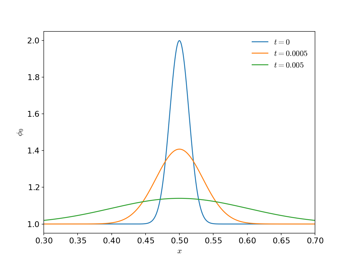
This shows the expected behavior—a strongly peaked concentration of \(\phi\) spreads out with time.