Fitting to a Line

Let’s consider the case of fitting data to a line. Our model has the form:

\[Y(x; a_1, a_2) = a_1 + a_2 x\]

and our fit appears as:

\[\chi^2(a_1, a_2) = \sum_{i=1}^N \frac{(a_1 + a_2 x_i - y_i)^2}{\sigma_i^2}\]

We want to minimize \(\chi^2(a_1, a_2)\).

We will actually care about the reduced chi-square, which is scaled by the number of degrees of freedom, \(N - M\), where \(N\) is the number of data points and \(M\) is the number of fitting parameters.

Tip

Generally we want the \(\chi^2 < 1\) for a fit to be considered “good”.

We start by differentiating with respect to the fit parameters and setting the derivatives to zero:

\[\begin{align*} \frac{\partial \chi^2}{\partial a_1} &= 2 \sum_{i=1}^{N} \frac{a_1 + a_2 x_i - y_i}{\sigma_i^2} = 0 \\ \frac{\partial \chi^2}{\partial a_2} &= 2 \sum_{i=1}^{N} \frac{a_1 + a_2 x_i - y_i}{\sigma_i^2} x_i= 0 \end{align*}\]

Separating the terms, we have:

\[\begin{align*} a_1 \sum_{i=1}^N \frac{1}{\sigma_i^2} + a_2 \sum_{i=1}^N \frac{x_i}{\sigma_i^2} - \sum_{i=1}^N \frac{y_i}{\sigma_i^2} &= 0 \\ a_1 \sum_{i=1}^N \frac{x_i}{\sigma_i^2} + a_2 \sum_{i=1}^N \frac{x_i^2}{\sigma_i^2} - \sum_{i=1}^N \frac{x_i y_i}{\sigma_i^2} &= 0 \end{align*}\]

This is a linear system with 2 equations and 2 unknowns.

Let’s define:

\[\begin{align*} C &= \sum_{i=1}^N \frac{1}{\sigma_i^2} \\ S_x &= \sum_{i=1}^N \frac{x_i}{\sigma_i^2} \\ S_y &= \sum_{i=1}^N \frac{y_i}{\sigma_i^2} \\ S_{x^2} &= \sum_{i=1}^N \frac{x_i^2}{\sigma_i^2} \\ S_{xy} &= \sum_{i=1}^N \frac{x_i y_i}{\sigma_i^2} \end{align*}\]

Then our system is:

\[\begin{align*} a_1 C + a_2 S_x - S_y &= 0 \\ a_1 S_x + a_2 S_{x^2} - S_{xy} &= 0 \end{align*}\]

We can solve this easily:

\[a_1 = \frac{S_{x^2} S_y - S_x S_{xy}}{C S_{x^2} - S_x^2}\]

\[a_2 = \frac{C S_{xy} - S_x S_y}{C S_{x^2} - S_x^2}\]

Example data

Let’s make some sample data that we perturb with Gaussian-normalized noise. We’ll use the numpy.random.randn() function. (Note, in C++, you can generate random numbers in a normal distribution via std::normal_distribution).

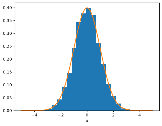
Let’s first see how this works. Let’s take a large number of samples and also plot a Gaussian distribution:

\[y(x) = \frac{1}{\sigma \sqrt{2\pi}} e^{-x^2/(2 \sigma^2)}\]

import numpy as np
import matplotlib.pyplot as plt

N = 10000
r = np.random.randn(N)

fig, ax = plt.subplots()
ax.hist(r, density=True, bins=20)

x = np.linspace(-5, 5, 200)
sigma = 1.0
ax.plot(x, np.exp(-x**2/(2*sigma**2)) / (sigma*np.sqrt(2.0*np.pi)), lw=2)
ax.set_xlabel("x")

Text(0.5, 0, 'x')

Now we can make some experimental data. This will be data that follows a line, but is perturbed by a Gaussian-normalized random number, to give it some experimental error.

def y_experiment(a1, a2, sigma, x):
    """ return the experimental data and error in a linear + random
    fashion; a1 is the intercept, a2 is the slope, and sigma is the
    error scale"""

    N = len(x)
    r = sigma * np.random.randn(N)

    return a1 + a2*x + r, np.abs(r)

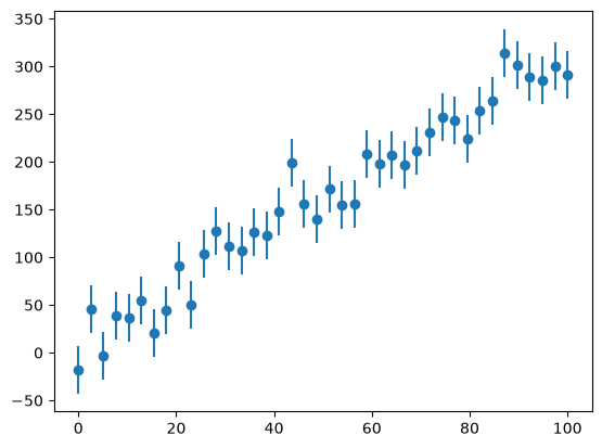
Now we can make the data that we want to fit to.

# number of data points
N = 40

# one-sigma error
sigma = 25.0

# independent variable
x = np.linspace(0.0, 100, N)

y, yerr = y_experiment(10.0, 3.0, sigma, x)

Let’s look at our “experiment”:

fig, ax = plt.subplots()
ax.errorbar(x, y, yerr=yerr, fmt="o")

<ErrorbarContainer object of 3 artists>

Now we can write a function to do the fitting

def linear_regression(x, y, yerr):
    """fit data (x_i, y_i) with errors {yerr_i} to a line"""
    
    N = len(x)

    C = np.sum(1.0 / yerr**2)

    S_x = np.sum(x / yerr**2)
    S_x2 = np.sum(x * x / yerr**2)

    S_y = np.sum(y / yerr**2)
    S_xy = np.sum(x * y / yerr**2)

    a2 = (C * S_xy - S_x * S_y)/(C * S_x2 - S_x**2)
    a1 = (S_y * S_x2 - S_xy * S_x) / (C * S_x2 - S_x**2)

    chisq = np.sum((a1 + a2 * x - y)**2 / yerr**2)
    chisq /= N-2

    return a1, a2, chisq

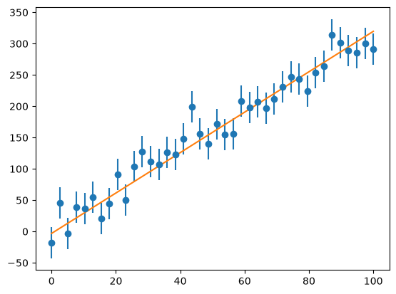
a1, a2, chisq = linear_regression(x, y, yerr)

Now we can look at how well our fit does:

ax.plot(x, a1 + a2*x)
fig

Pathologies

We need to be careful to not over-interpret a fit. Consider the Anscombe’s quartet. These 4 very different datasets all have the same linear fit (to a few digits significance).