
Fast Fourier Transform#
So far we have been working with the discrete Fourier transform (DFT). This does what we want, but its complexity scales like \(\mathcal{O}(N^2)\), so for really large datasets, it will be slow.
Note
The fast Fourier transform (FFT) is algebraically identical to the DFT, but uses some clever tricks to speed up the computation, resulting in an algorithm that scales like \(\mathcal{O}(N\log N)\).
The standard algorithm for the FFT is the Cooley-Tukey FFT. Not only does it gain speed from a divide-and-conquer algorithm, it also does the transform in-place, saving memory.
Note
We’ll only focus on the performance improvement here.
The FFT can be written as:
where we simply split the even and odd terms.
Now look at the even terms:
This is just the DFT of the \(N/2\) even samples.
The odd terms are:
Here, \(O_k\) is just the DFT of the \(N/2\) odd samples
If we define:
then we can write our original transform as:
In doing this, we went from one DFT involving \(N\) samples to 2 DFTs with \(N/2\) samples. The number of wavenumbers also is cut in half.
Periodicity tells us that:
since \(E_k\) and \(O_k\) are periodic with \(N/2\)
Let’s consider 8 samples:
Express this in terms of the FFTs of the even and odd terms:
\[F_k = \mathcal{F}(f_0, f_2, f_4, f_6) + \omega^k \mathcal{F}(f_1, f_3, f_5, f_7)\]this is defined for \(k = 0, 1, 2, 3\), since that’s what each of the \(N/2\) samples gets.
The 2nd half of the frequencies are:
\[F_{k+N/2} = \mathcal{F}(f_0, f_2, f_4, f_6) - \omega^k \mathcal{F}(f_1, f_3, f_5, f_7)\]This gives \(k = 4, 5, 6, 7\)
So 2 FFTs of 4 samples each gives us the FFT of 8 samples defined over 8 wavenumbers.
We then apply this recursively.
We eventually get down to \(N\) FFTs of 1 sample each:
Warning
The procedure that we outlined above (and implement below) assumes that the number of data points is a power of 2.
Implementation#
import numpy as np
import matplotlib.pyplot as plt
def fft(f_n):
    """ perform a discrete Fourier transform.  We use the same
        conventions as NumPy's FFT

        here,

              N-1         -2 pi i n k /N
        F_k = sum  f   exp
              i=0   n

    """

    N = len(f_n)

    if N == 1:
        return f_n
    else:

        # split into even and odd and find the FFTs of each half
        f_even = f_n[0:N:2]
        f_odd = f_n[1:N:2]

        F_even = fft(f_even)
        F_odd = fft(f_odd)

        # combine them.  Each half has N/2 wavenumbers, but due to
        # periodicity, we can compute N wavenumbers
        omega = np.exp(-2*np.pi*1j/N)

        # allocate space for the frequency components -- they are,
        # in general, complex
        F_k = np.zeros((N), dtype=np.complex128)

        oterm = omega**np.arange(N//2)
        F_k[0:N//2] = F_even + oterm * F_odd
        F_k[N//2:] = F_even - oterm * F_odd

    return F_k
We’ll also copy over our DFT:
def dft(f_n):
    """perform a discrete Fourier transform"""

    N = len(f_n)
    n = np.arange(N)

    f_k = np.zeros((N), dtype=np.complex128)

    for k in range(N):
        f_k[k] = np.sum(f_n * np.exp(-2.0 * np.pi * 1j * n * k / N))
    return f_k
Testing#
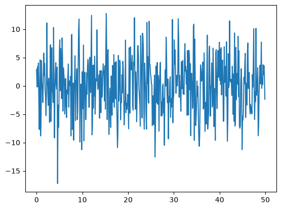
Let’s create some random data and compare our FFT against our DFT.
def data(xmin=0.0, xmax=50.0, npts=32):
    """create a multi-frequency, multi-phase sine dataset"""

    xx = np.linspace(0.0, xmax, npts, endpoint=False)

    # number of frequencies to superpose
    nfreq = 48

    # frequency in terms of 1/length
    freqs = np.random.randint(1, npts, nfreq) / xmax
    phases = np.random.uniform(0.0, 2.0*np.pi, nfreq)

    f_n = np.zeros_like(xx)
    for f, p in zip(freqs, phases):
        f_n += np.sin(2.0*np.pi*f*xx + p)

    return xx, f_n
xmax = 50.0
xx, f_n = data(xmax=xmax, npts=512)
fig, ax = plt.subplots()

ax.plot(xx, f_n)
[<matplotlib.lines.Line2D at 0x7f817f287230>]
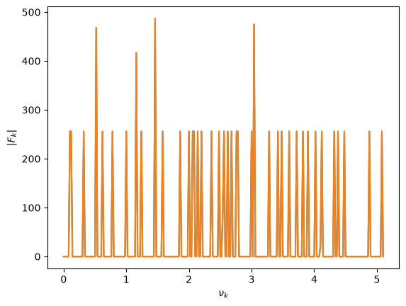
Let’s ensure they get the same answer
f_k_dft = dft(f_n)
f_k_fft = fft(f_n)

N = len(f_k_dft)
k = np.arange(N) / xmax
fig, ax = plt.subplots()

ax.plot(k[:N//2], np.abs(f_k_dft[:N//2]))
ax.plot(k[:N//2], np.abs(f_k_fft[:N//2]))

ax.set_xlabel(r"$\nu_k$")
ax.set_ylabel(r"$|F_k|$")
Text(0, 0.5, '$|F_k|$')
Performance#
Now let’s time them
import time
Ns = [2, 4, 8, 16, 32, 64, 128, 256, 512, 1024, 2048, 4096, 8192, 16384]

dft_times = []
fft_times = []

for N in Ns:
    xx, f_n = data(npts=N)

    start = time.perf_counter()
    f_k_dft = dft(f_n)
    dft_times.append(time.perf_counter() - start)

    start = time.perf_counter()
    f_k_fft = fft(f_n)
    fft_times.append(time.perf_counter() - start)

fig, ax = plt.subplots()

ax.scatter(Ns, dft_times, label="DFT")
ax.scatter(Ns, fft_times, label="FFT")
ax.legend()
ax.set_xscale("log")
ax.set_yscale("log")
ax.set_xlabel("N")
ax.set_ylabel("computational time (s)")
ax.grid()
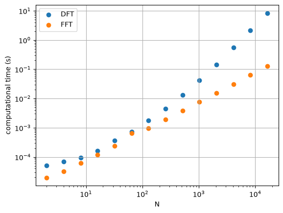
We see that the FFT version is much faster for large \(N\)