Application: X-ray Burst Timing

The Rossi X-ray Timing Explorer (RXTE) has very high time resolution and has been used to observe a large number of X-ray sources. We’ll look at the data from the low-mass X-ray binary 4U 1728-34—this is an X-ray burst system.

In Strohmayer et al. 1996 it was shown that the neutron star spin rate can be seen in the Fourier transform of the lightcurve of the burst. Here we repeat the analysis.

We thank Tod Strohmayer for sharing the data from that paper: 4u1728_burstdata.txt

Note

Although the data is stored in a multidimensional fashion in the file, it is actually a time-series. We’ll flatten the data into a 1-d array when we read.

import numpy as np
import matplotlib.pyplot as plt

data = np.loadtxt("4u1728_burstdata.txt").flatten()

N = len(data)
N

262144

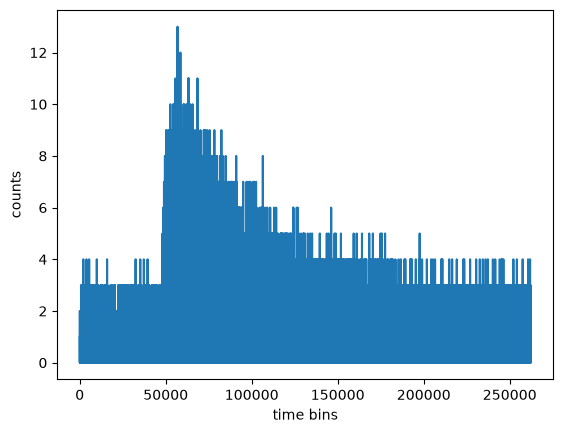
We can start out by plotting all of the data.

fig, ax = plt.subplots()
ax.plot(data)

[<matplotlib.lines.Line2D at 0x7f27d8f46910>]

We’ll bin the data into fewer samples to build up the signal to noise.

Tip

We can do this by reshaping it into a 2-d array and then summing over the columns.

binned_data = data.reshape(N // 256, 256).sum(axis=1)

fig, ax = plt.subplots()
ax.plot(binned_data)

[<matplotlib.lines.Line2D at 0x7f27d8b24550>]

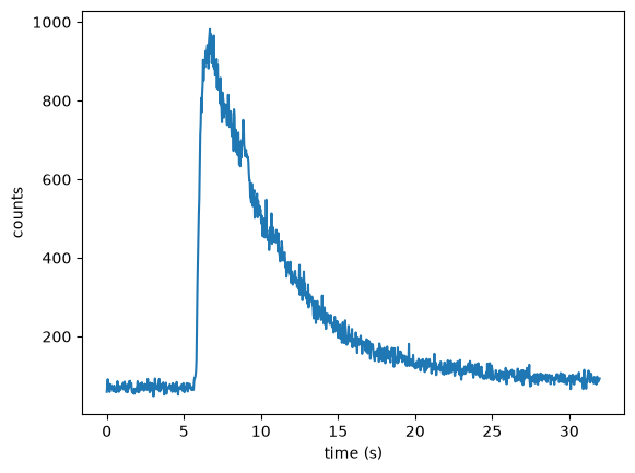
Now we see a much clearer X-ray lightcurve. This looks very similar to Figure 1 in Stohmayer et al. 1996.

Next we want to take the FFT and look to see if there are any interesting frequencies with a lot of power

c_k = np.fft.rfft(data)

We want to get the physical frequencies corresponding to the Fourier coefficients

The data encompasses 32 s (and with 262144 points, has a sampling rate of 1/8192 s).

T = 32.0
kfreq = np.fft.rfftfreq(N) * N / T

Now we can plot the power spectrum. We normalize by \(2/N\)

fig, ax = plt.subplots()
ax.plot(kfreq, np.abs(c_k)**2 * 2 / N)

ax.set_xscale("log")
ax.set_yscale("log")

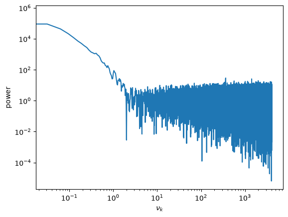
Here we see a signal around 300 Hz. We’ll bin the Fourier data to increase the signal to noise. The original paper did this by a factor of 8.

c_k_binned = np.abs(c_k[1:]).reshape(int(len(c_k)//8), 8).mean(axis=1)
kfreq_binned = kfreq[1:].reshape(int(len(kfreq)//8), 8).mean(axis=1)

fig, ax = plt.subplots()
ax.plot(kfreq_binned, c_k_binned**2 * 2 / N)
ax.set_xscale("log")
ax.set_yscale("log")

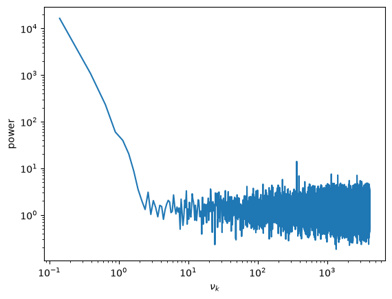
Now we see the strong signal at around 363 Hz—this is the same frequency identified as the neutron star rotation rate in the original paper.

We can zoom in on the peak around 300 Hz

ax.set_xscale("linear")
ax.set_yscale("linear")

ax.set_xlim(340, 380)
ax.set_ylim(0, 20)

fig

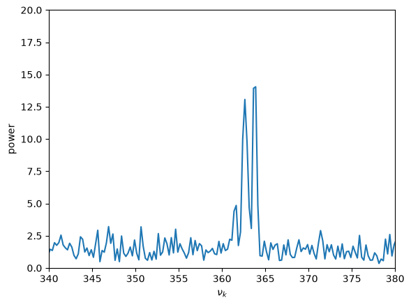
This shows a clear peak around 363 Hz, matching the inset in Figure 1 of Strohmayer et al. 1996. This was identified as the rotation rate of the neutron star.