Application: Galaxy Classification with Keras

Now we’ll try to do the galaxy classification with Keras. This will allow us to explore more features in the network.

In particular we’ll use a convolutional neural network.

import numpy as np
import matplotlib.pyplot as plt
import h5py

We’ll need the Galaxy class we defined earlier.

galaxy_types = {0: "disturbed galaxies",
                1: "merging galaxies",
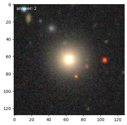
                2: "round smooth galaxies",
                3: "in-between round smooth galaxies",
                4: "cigar shaped smooth galaxies",
                5: "barred spiral galaxies",
                6: "unbarred tight spiral galaxies",
                7: "unbarred loose spiral galaxies",
                8: "edge-on galaxies without bulge",
                9: "edge-on galaxies with bulge"}

class Galaxy:
    def __init__(self, data, answer, *, index=-1):
        self.data = np.array(data, dtype=np.float32) / 255.0
        self.answer = answer

        self.index = index

    def plot(self, ax=None):
        if ax is None:
            fig, ax = plt.subplots()
        ax.imshow(self.data, interpolation="nearest")
        ax.text(0.025, 0.95, f"answer: {self.answer}",
                color="white", transform=ax.transAxes)

    def validate(self, prediction):
        """check if a categorical prediction matches the answer"""
        return np.argmax(prediction) == self.answer

A data manager class

We’ll create a class to manage access to the data. This is similar to the version in our “from scratch” implementation, except we provide a generator to Keras.

This will do the following:

• open the file and store the handles to access the data

• partition the data into test and training sets

• provide a means to shuffle the data

• provide a generator to get the next batch of training data

• allow us to coarsen the images to a reduced resolution to make the training easier.

Tip

We will read all of the data once, which will take about 3.5 GB of memory. It is kept as a uint8 until needed.

from keras.utils import to_categorical

class DataManager:
    def __init__(self, partition=0.8,
                 batch_size=32,
                 datafile="Galaxy10_DECals.h5",
                 coarsen=1):
        """manage access to the data

        partition: fraction that should be training
        datafile: name of the hdf5 file with the data
        coarsen: reduce the number of pixels by this factor
        """

        self.ds = h5py.File(datafile)
        self.ans = np.array(self.ds["ans"])
        self.images = np.array(self.ds["images"])

        self.coarsen = coarsen

        self.batch_size = batch_size
        
        N = len(self.ans)

        # create a set of indices for the galaxies and randomize
        self.indices = np.arange(N, dtype=np.uint32)
        self.rng = np.random.default_rng()
        self.rng.shuffle(self.indices)

        # partition into training and test sets
        # these indices will always refer to the index in the original
        # unsplit dataset
        n_cut = int(partition * N)

        # we want this to be a multiple of the batch size
        n_cut -= n_cut % self.batch_size

        self.training_indices = self.indices[0:n_cut]
        self.test_indices = self.indices[n_cut:N]

        self.n_training = len(self.training_indices)
        self.n_test = len(self.test_indices)

        # number of batches for the training
        self.n_batches = n_cut // self.batch_size

        # shape information
        self.input_shape = self._get_galaxy(0).data.shape
    
    def _get_galaxy(self, index):
        """return a numpy array containing a single galaxy image, coarsened
        if necessary by averaging"""
        _tmp = self.images[index, :, :, :]
        if self.coarsen > 1:
            _tmp = np.mean(_tmp.reshape(_tmp.shape[0]//self.coarsen, self.coarsen,
                                        _tmp.shape[1]//self.coarsen, self.coarsen,
                                        _tmp.shape[2]), axis=(1, 3))
        return _tmp

    def training_images(self):
        self.reset_training()
        for idx in self.training_indices:
            yield Galaxy(self._get_galaxy(idx), self.ans[idx], index=idx)

    def batched_training_generator(self):
        while True:
            self.reset_training()
            batch_x = []
            batch_y = []
            for idx in self.training_indices:
                g = Galaxy(self._get_galaxy(idx), self.ans[idx], index=idx)
                batch_x.append(g.data)
                batch_y.append(to_categorical(g.answer, 10))

                if len(batch_x) == self.batch_size:
                    yield (np.array(batch_x), np.array(batch_y))
                    batch_x = []
                    batch_y = []
    
    def reset_training(self):
        """prepare for the next epoch: shuffle the training data and
        reset the index to point to the start"""
        self.rng.shuffle(self.training_indices)

    def testing_images(self):
        for idx in self.test_indices:
            yield Galaxy(self._get_galaxy(idx), self.ans[idx], index=idx)

Tip

The training_images() and testing_images() are generators (like range()), so we can iterate like:

d = DataManager()
for g in d.training_images():
    # do stuff with g

and g is only converted to 32-bit float as needed.

Here we create a DataManager that will coarsen the images by a factor of 4 (so they will be 64x64 pixels with 3 colors). We also need to specify the batch size.

d = DataManager(coarsen=2, batch_size=128)

for n, (x, y) in enumerate(d.batched_training_generator()):
    print(x.shape)
    break

(128, 128, 128, 3)

d.input_shape

(128, 128, 3)

we can see how many images there are in the training and test sets

d.n_training, d.n_test

(14080, 3656)

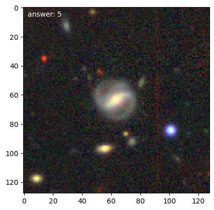
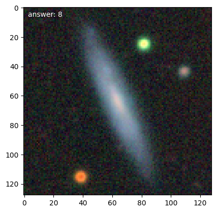
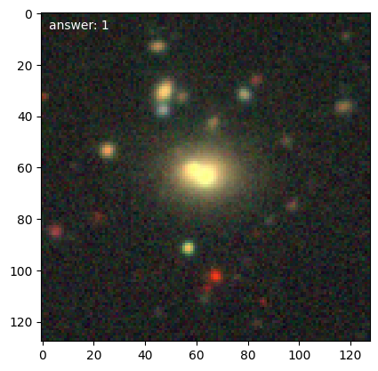
We can then get loop over training galaxies and look at them (we’ll break after 5):

for n, g in enumerate(d.training_images()):
    g.plot()
    if n == 4:
        break

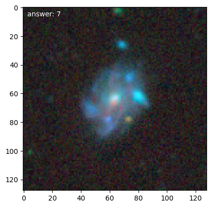
Note

Each time we access the generator it randomizes the galaxies in the training set.

Implementing our neural network

We’ll use just a single hidden layer. If we use more hidden layers, then there are so many parameters that we will need to do a lot of training (epochs).

Tip

Our DataManager will tell us the size of the input layer, the number of batches, the batch size, etc.

from keras.models import Sequential
from keras.layers import Input, Dense, Dropout, Conv2D, MaxPooling2D, Flatten

model = Sequential()
model.add(Input(shape=d.input_shape))
model.add(Conv2D(32, kernel_size=(3, 3), activation="relu"))
model.add(MaxPooling2D(pool_size=(2, 2)))
model.add(Conv2D(64, kernel_size=(3, 3), activation="relu"))
model.add(MaxPooling2D(pool_size=(2, 2)))
model.add(Conv2D(64, kernel_size=(3, 3), activation="relu"))
model.add(MaxPooling2D(pool_size=(2, 2)))
model.add(Flatten())
model.add(Dense(10, activation="softmax"))

model.summary()

Model: "sequential_3"

┏━━━━━━━━━━━━━━━━━━━━━━━━━━━━━━━━━┳━━━━━━━━━━━━━━━━━━━━━━━━┳━━━━━━━━━━━━━━━┓
┃ Layer (type)                    ┃ Output Shape           ┃       Param # ┃
┡━━━━━━━━━━━━━━━━━━━━━━━━━━━━━━━━━╇━━━━━━━━━━━━━━━━━━━━━━━━╇━━━━━━━━━━━━━━━┩
│ conv2d_7 (Conv2D)               │ (None, 126, 126, 32)   │           896 │
├─────────────────────────────────┼────────────────────────┼───────────────┤
│ max_pooling2d_7 (MaxPooling2D)  │ (None, 63, 63, 32)     │             0 │
├─────────────────────────────────┼────────────────────────┼───────────────┤
│ conv2d_8 (Conv2D)               │ (None, 61, 61, 64)     │        18,496 │
├─────────────────────────────────┼────────────────────────┼───────────────┤
│ max_pooling2d_8 (MaxPooling2D)  │ (None, 30, 30, 64)     │             0 │
├─────────────────────────────────┼────────────────────────┼───────────────┤
│ conv2d_9 (Conv2D)               │ (None, 28, 28, 64)     │        36,928 │
├─────────────────────────────────┼────────────────────────┼───────────────┤
│ max_pooling2d_9 (MaxPooling2D)  │ (None, 14, 14, 64)     │             0 │
├─────────────────────────────────┼────────────────────────┼───────────────┤
│ flatten_3 (Flatten)             │ (None, 12544)          │             0 │
├─────────────────────────────────┼────────────────────────┼───────────────┤
│ dense_3 (Dense)                 │ (None, 10)             │       125,450 │
└─────────────────────────────────┴────────────────────────┴───────────────┘

 Total params: 181,770 (710.04 KB)

 Trainable params: 181,770 (710.04 KB)

 Non-trainable params: 0 (0.00 B)

We’ll use a different optimizer now, the Adam optimizer. This is supposed to be one of the best that Keras provides.

from keras.optimizers import Adam

rms = Adam()
model.compile(loss='categorical_crossentropy',
              optimizer=rms, metrics=['accuracy'])

The keras fit() method can work with a generator directly, so we just pass in the generator.

model.fit(d.batched_training_generator(),
          batch_size=d.batch_size,
          steps_per_epoch=d.n_batches,
          epochs=20)

Epoch 1/20
110/110 ━━━━━━━━━━━━━━━━━━━━ 98s 896ms/step - accuracy: 0.2091 - loss: 2.1281
Epoch 2/20
110/110 ━━━━━━━━━━━━━━━━━━━━ 100s 908ms/step - accuracy: 0.4391 - loss: 1.5734
Epoch 3/20
110/110 ━━━━━━━━━━━━━━━━━━━━ 103s 932ms/step - accuracy: 0.5361 - loss: 1.3256
Epoch 4/20
110/110 ━━━━━━━━━━━━━━━━━━━━ 101s 921ms/step - accuracy: 0.5861 - loss: 1.1807
Epoch 5/20
110/110 ━━━━━━━━━━━━━━━━━━━━ 104s 944ms/step - accuracy: 0.6242 - loss: 1.0776
Epoch 6/20
110/110 ━━━━━━━━━━━━━━━━━━━━ 101s 913ms/step - accuracy: 0.6728 - loss: 0.9610
Epoch 7/20
110/110 ━━━━━━━━━━━━━━━━━━━━ 102s 930ms/step - accuracy: 0.7200 - loss: 0.8336
Epoch 8/20
110/110 ━━━━━━━━━━━━━━━━━━━━ 101s 918ms/step - accuracy: 0.7374 - loss: 0.7848
Epoch 9/20
110/110 ━━━━━━━━━━━━━━━━━━━━ 104s 945ms/step - accuracy: 0.7601 - loss: 0.7158
Epoch 10/20
110/110 ━━━━━━━━━━━━━━━━━━━━ 107s 970ms/step - accuracy: 0.7812 - loss: 0.6392
Epoch 11/20
110/110 ━━━━━━━━━━━━━━━━━━━━ 103s 941ms/step - accuracy: 0.8107 - loss: 0.5757
Epoch 12/20
110/110 ━━━━━━━━━━━━━━━━━━━━ 102s 932ms/step - accuracy: 0.8315 - loss: 0.5247
Epoch 13/20
110/110 ━━━━━━━━━━━━━━━━━━━━ 104s 943ms/step - accuracy: 0.8612 - loss: 0.4346
Epoch 14/20
110/110 ━━━━━━━━━━━━━━━━━━━━ 107s 973ms/step - accuracy: 0.8747 - loss: 0.3981
Epoch 15/20
110/110 ━━━━━━━━━━━━━━━━━━━━ 106s 962ms/step - accuracy: 0.8864 - loss: 0.3385
Epoch 16/20
110/110 ━━━━━━━━━━━━━━━━━━━━ 108s 977ms/step - accuracy: 0.9007 - loss: 0.3162
Epoch 17/20
110/110 ━━━━━━━━━━━━━━━━━━━━ 106s 966ms/step - accuracy: 0.9142 - loss: 0.2689
Epoch 18/20
110/110 ━━━━━━━━━━━━━━━━━━━━ 107s 968ms/step - accuracy: 0.9259 - loss: 0.2297
Epoch 19/20
110/110 ━━━━━━━━━━━━━━━━━━━━ 103s 940ms/step - accuracy: 0.9375 - loss: 0.1989
Epoch 20/20
110/110 ━━━━━━━━━━━━━━━━━━━━ 103s 938ms/step - accuracy: 0.9438 - loss: 0.1798

<keras.src.callbacks.history.History at 0x7fdbc2513a10>

for g in d.testing_images():
    print(np.expand_dims(g.data, axis=0).shape)
    break

(1, 128, 128, 3)

n_correct = 0
for g in d.testing_images():
    res = model.predict(np.expand_dims(g.data, axis=0), verbose=0)
    if np.argmax(res) == g.answer:
        n_correct += 1
print(f"fraction correct = {n_correct / d.n_test}")

fraction correct = 0.5804157549234136