2nd Order Runge-Kutta / Midpoint Method

We’ll continue to work on the orbit problem.

Note

To make life easier, the OrbitState and rhs functions are now in a module, along with a function initial_conditions() that provides the initial state, plot() that makes a plot of the orbit, and error() that computes the error. We can simply do

import orbit_util as ou

to access these (e.g., as ou.plot()).

The source for orbit_util is here: orbit_util.py

Here’s what this module looks like:

import numpy as np
import matplotlib.pyplot as plt

GM = 4*np.pi**2

class OrbitState:
    # a container to hold the star positions
    def __init__(self, x, y, u, v):
        self.x = x
        self.y = y
        self.u = u
        self.v = v

    def __add__(self, other):
        return OrbitState(self.x + other.x, self.y + other.y,
                          self.u + other.u, self.v + other.v)

    def __sub__(self, other):
        return OrbitState(self.x - other.x, self.y - other.y,
                          self.u - other.u, self.v - other.v)

    def __mul__(self, other):
        return OrbitState(other * self.x, other * self.y,
                          other * self.u, other * self.v)

    def __rmul__(self, other):
        return self.__mul__(other)

    def __str__(self):
        return f"{self.x:10.6f} {self.y:10.6f} {self.u:10.6f} {self.v:10.6f}"

def rhs(state):
    """ RHS of the equations of motion."""

    # current radius
    r = np.sqrt(state.x**2 + state.y**2)

    # position
    xdot = state.u
    ydot = state.v

    # velocity
    udot = -GM * state.x / r**3
    vdot = -GM * state.y / r**3

    return OrbitState(xdot, ydot, udot, vdot)

def initial_conditions():
    x0 = 0
    y0 = 1
    u0 = -np.sqrt(GM / y0)
    v0 = 0

    return OrbitState(x0, y0, u0, v0)

def plot(history, ax=None, label=None):
    """make a plot of the solution.  If ax is None we setup a figure
    and make the entire plot returning the figure object, otherwise, we
    just append the plot to a current axis"""

    fig = None

    if ax is None:
        fig = plt.figure()
        ax = fig.add_subplot(111)

        # draw the Sun
        ax.scatter([0], [0], marker=(20,1), color="y", s=250)

    # draw the orbit
    xs = [q.x for q in history]
    ys = [q.y for q in history]

    ax.plot(xs, ys, label=label)

    if fig is not None:
        ax.set_aspect("equal")
        ax.set_xlabel("x [AU]")
        ax.set_ylabel("y [AU]")

    return fig

def error_radius(history):

    # define the error to be distance from (0, 0) at end compared to start
    R_orig = np.sqrt(history[0].x**2 + history[0].y**2)
    R_new = np.sqrt(history[-1].x**2 + history[-1].y**2)
    e = np.abs(R_new - R_orig)

    return e

def error_position(history):
    """return the difference in the distance from the Sun"""
    dx = history[0].x - history[-1].x
    dy = history[0].y - history[-1].y
    return np.sqrt(dx**2 + dy**2)

import numpy as np
import matplotlib.pyplot as plt

import orbit_util as ou

The Euler method was based on a first-order difference approximation to the derivative. But we know that a centered-derivative is second order accurate, so we can try to update our system in the form:

\[\frac{{\bf r}^{n+1} - {\bf r}^n}{\tau} = {\bf v}^{n+1/2} + \mathcal{O}(\tau^2)\]

\[\frac{{\bf v}^{n+1} - {\bf v}^n}{\tau} = {\bf a}^{n+1/2} + \mathcal{O}(\tau^2)\]

Then the updates are:

\[{\bf r}^{n+1} = {\bf r}^n + \tau \, {\bf v}^{n+1/2} + \mathcal{O}(\tau^3)\]

\[{\bf v}^{n+1} = {\bf v}^n + \tau \, {\bf a}^{n+1/2} + \mathcal{O}(\tau^3)\]

This is locally third-order accurate (but globally second-order accurate), but we don’t know how to compute the state at the half-time.

To find the \(n+1/2\) state, we first use Euler’s method to predict the state at the midpoint in time. We then use this provisional state to evaluate the accelerations at the midpoint and use those to update the state fully through \(\tau\).

The two step process appears as:

\[{\bf r}^\star = {\bf r}^n + (\tau / 2) {\bf v}^n\]

\[{\bf v}^\star = {\bf v}^n + (\tau / 2) {\bf a}^n\]

then we use this for the full update:

\[{\bf r}^{n+1} = {\bf r}^n + \tau \, {\bf v}^\star\]

\[{\bf v}^{n+1} = {\bf v}^n + \tau \, {\bf a}({\bf r}^\star)\]

This is called the midpoint method or 2nd-order Euler’s method.

Graphically this looks like the following:

First step

First we take a half step and we evaluate the slope at the midpoint:

Final update

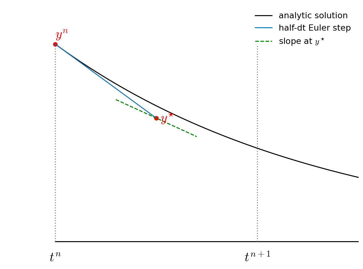
Then we go back to \(t^n\) but follow the slope we found above all the way to \(t^{n+1}\):

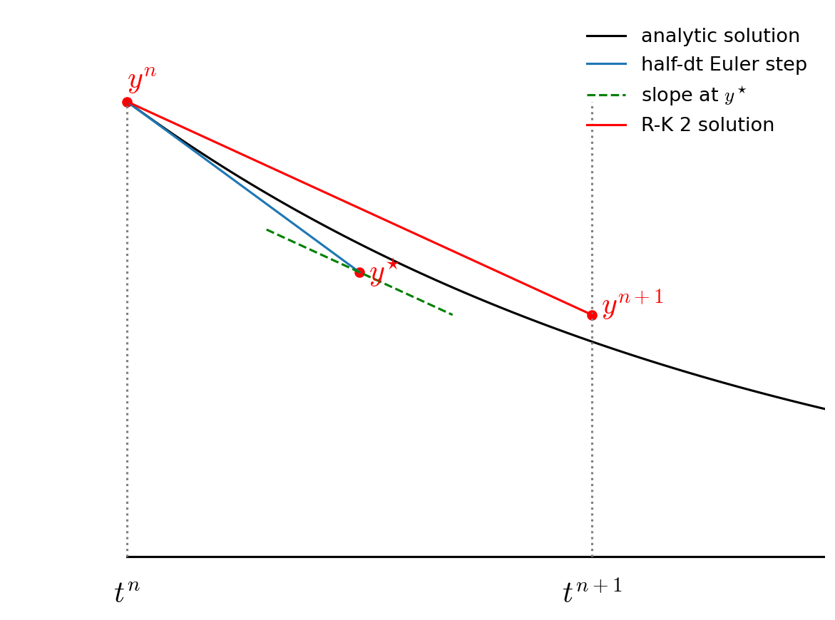
Notice how the final step (the red line) is parallel to the slope we computed at \(t^{n+1/2}\). Also note that the solution at \(t^{n+1}\) is much closer to the analytic solution than in the figure from Euler’s method.

Implementation

Let’s see how this method does with the orbit problem.

def int_rk2(state0, tau, T):

    times = []
    history = []
    
    # initialize time
    t = 0
    
    # store the initial conditions
    times.append(t)
    history.append(state0)
    
    # main timestep loop
    while t < T:
        
        state_old = history[-1]
        
        # make sure that the last step does not take us past T
        tau = min(tau, T - t)

        # get the RHS
        ydot = ou.rhs(state_old)
    
        # predict the state at the midpoint
        state_tmp = state_old + 0.5 * tau * ydot
        
        # evaluate the RHS at the midpoint
        ydot = ou.rhs(state_tmp)
        
        # do the final update
        state_new = state_old + tau * ydot
        t += tau
        
        # store the state
        times.append(t)
        history.append(state_new)
        
    return times, history

Note

Our int_rk2() function is almost identical to our first-order Euler implementation. There are actually only 2 lines that are different:

        # predict the state at the midpoint
        state_tmp = state_old + 0.5 * tau * ydot
        
        # evaluate the RHS at the midpoint
        ydot = ou.rhs(state_tmp)

Testing

Integrate our orbit.

T = 1
tau = T/12.0

state0 = ou.initial_conditions()

times, history = int_rk2(state0, tau, 1)

Let’s plot our orbit

fig = ou.plot(history)

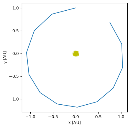
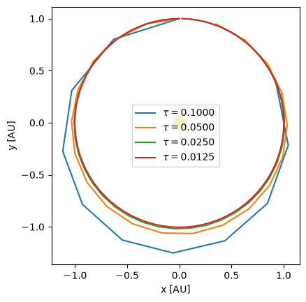
This is substantially better than the first-order Euler method. Now let’s look at a range of timesteps.

taus = [0.1, 0.05, 0.025, 0.0125]

for n, tau in enumerate(taus):
    times, history = int_rk2(state0, tau, 1)
    
    if n == 0:
        fig = ou.plot(history, label=rf"$\tau = {tau:6.4f}$")
    else:
        ou.plot(history, ax=fig.gca(), label=rf"$\tau = {tau:6.4f}$")
        
fig.gca().legend()

<matplotlib.legend.Legend at 0x7efd100f0550>

Convergence

How does the error converge?

for tau in [0.1, 0.05, 0.025, 0.0125, 0.00625]:
    times, history = int_rk2(state0, tau, 1)
    print(f"{tau:8} : {ou.error_radius(history):10.5g} {ou.error_position(history):10.5g}")

     0.1 :     0.0116     1.0856
    0.05 :   0.011123    0.35694
   0.025 :  0.0024709   0.096669
  0.0125 : 0.00036069   0.023906
 0.00625 : 4.6926e-05  0.0058463

Notice that once we get past the first, very coarse \(\tau\), the errors seem to decrease by a factor of 4 when we halve the timestep—as we’d expect for a 2nd order accurate method. (Actually, it looks like the measure of radius converges better than position).