
Residual#
We need to have a way to tell when to stop smoothing.
If we know the analytic solution, then we can just compare to that, and keep iterating until the error is small, but that kinda defeats the purpose.
Instead, we can measure how well we satisfy the discrete equation—this is called the residual.
We still need something to compare to, so we define the source norm, \(\| f \|\), and we will pick a tolerance \(\epsilon\) and iterate until:
For the special case of a homogeneous source (\(f = 0\)), then we will iterate until
We will use the L2 norm:
Implementation#
Let’s update our grid class to include a norm and residual function:
import numpy as np
import matplotlib.pyplot as plt
This is the same grid class as before
class Grid:
    def __init__(self, nx, ng=1, xmin=0, xmax=1,
                 bc_left_type="dirichlet", bc_left_val=0.0,
                 bc_right_type="dirichlet", bc_right_val=0.0):

        self.xmin = xmin
        self.xmax = xmax
        self.ng = ng
        self.nx = nx

        self.bc_left_type = bc_left_type
        self.bc_left_val = bc_left_val

        self.bc_right_type = bc_right_type
        self.bc_right_val = bc_right_val

        # python is zero-based.  Make easy integers to know where the
        # real data lives
        self.ilo = ng
        self.ihi = ng+nx-1

        # physical coords -- cell-centered
        self.dx = (xmax - xmin)/(nx)
        self.x = xmin + (np.arange(nx+2*ng)-ng+0.5)*self.dx

        # storage for the solution
        self.phi = self.scratch_array()
        self.f = self.scratch_array()

    def scratch_array(self):
        """return a scratch array dimensioned for our grid """
        return np.zeros((self.nx+2*self.ng), dtype=np.float64)

    def norm(self, e):
        """compute the L2 norm of e that lives on our grid"""
        return np.sqrt(self.dx * np.sum(e[self.ilo:self.ihi+1]**2))

    def fill_bcs(self):
        """fill the boundary conditions on phi"""

        # we only deal with a single ghost cell here

        # left
        if self.bc_left_type.lower() == "dirichlet":
            self.phi[self.ilo-1] = 2 * self.bc_left_val - self.phi[self.ilo]
        elif self.bc_left_type.lower() == "neumann":
            self.phi[self.ilo-1] = self.phi[self.ilo] - self.dx * self.bc_left_val
        else:
            raise ValueError("invalid bc_left_type")

        # right
        if self.bc_right_type.lower() == "dirichlet":
            self.phi[self.ihi+1] = 2 * self.bc_right_val - self.phi[self.ihi]
        elif self.bc_right_type.lower() == "neumann":
            self.phi[self.ihi+1] = self.phi[self.ihi] - self.dx * self.bc_right_val
        else:
            raise ValueError("invalid bc_right_type")
Now we’ll write our residual routine
def residual_norm(g):
    """compute the residual norm"""
    r = g.scratch_array()
    r[g.ilo:g.ihi+1] = g.f[g.ilo:g.ihi+1] - (g.phi[g.ilo+1:g.ihi+2] -
                                            2 * g.phi[g.ilo:g.ihi+1] +
                                            g.phi[g.ilo-1:g.ihi]) / g.dx**2
    return g.norm(r)
Now we’ll write a relaxation function that does smoothing until either a maximum number of iterations is taken or we reach a desired tolerance. If the tolerance is set to None, then the routine will take the full amount of iterations.
class TooManyIterations(Exception):
    pass

def relax(g, tol=1.e-8, max_iters=200000, analytic=None):

    iter = 0
    fnorm = g.norm(g.f)

    # if the RHS is f = 0, then set the norm to 1
    # this ensures that we then check for residual < eps
    if fnorm == 0.0:
        fnorm = 1

    g.fill_bcs()
    r = residual_norm(g)

    res_norm = []
    true_norm = []

    while iter < max_iters and (tol is None or r > tol * fnorm):

        g.phi[g.ilo:g.ihi+1:2] = 0.5 * (-g.dx * g.dx * g.f[g.ilo:g.ihi+1:2] +
                                        g.phi[g.ilo+1:g.ihi+2:2] + g.phi[g.ilo-1:g.ihi:2])

        g.fill_bcs()

        g.phi[g.ilo+1:g.ihi+1:2] = 0.5 * (-g.dx * g.dx * g.f[g.ilo+1:g.ihi+1:2] +
                                          g.phi[g.ilo+2:g.ihi+2:2] + g.phi[g.ilo:g.ihi:2])

        g.fill_bcs()

        r = residual_norm(g)
        res_norm.append(r / fnorm)

        if analytic is not None:
            true_norm.append(g.norm(g.phi - analytic(g.x)))

        iter += 1

    if tol is not None and iter >= max_iters:
        raise TooManyIterations(f"too many iterations, niter = {iter}")

    return res_norm, true_norm, iter
Residual vs. Truncation Error#
Let’s look at how the residual error compares to the truncation error of our discretization. We’ll take a fixed number of iterations for our same model problem,
on \([0, 1]\) with homogeneous Dirichlet BCs.
def analytic(x):
    return -np.sin(x) + x * np.sin(1.0)

def f(x):
    return np.sin(x)
from matplotlib.lines import Line2D
fig, ax = plt.subplots()

for i, nx in enumerate([16, 32, 64]):
    g = Grid(nx)
    g.f[:] = f(g.x)

    res_norm, true_norm, _ = relax(g, tol=None, max_iters=20000, analytic=analytic)
    n = np.arange(len(res_norm)) + 1

    ax.loglog(n, true_norm, label=f"{nx}", color=f"C{i}")
    ax.loglog(n, res_norm, ls=":", color=f"C{i}")

    print(f"nx = {nx}, true error = {true_norm[-1]}")

# manually add line types to the legend
handles, labels = ax.get_legend_handles_labels()
line1 = Line2D([0], [0], ls="-", color="k", label="truncation error")
line2 = Line2D([0], [0], ls=":", color="k", label="residual")
handles.extend([line1, line2])
ax.legend(handles=handles, ncol=2)

ax.set_xlabel("number of smoothing iterations")
ax.grid(ls=":", color="0.5")
nx = 16, true error = 0.0002489743563076079
nx = 32, true error = 6.22480653738797e-05
nx = 64, true error = 1.5562295551083177e-05
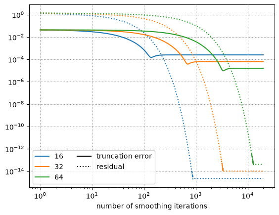
Look at what this shows us:
The truncation error (solid line) stalls at a much higher value than the residual (dotted).
The truncation error converges second order with the number of zones (look at the numbers printed during the run)
As we increase the number of zones, we need more iterations until the residual drops to machine roundoff
The residual error eventually reaches roundoff—this indicates that we satisfy the discrete equation “exactly”
Important
The residual is telling us how well we satisfy the discrete form of Poisson’s equation, but it is not telling us anything about whether the discrete approximation we are using for Poisson’s equation is a good approximation. That is our job as a computational scientist to assess.
We are using a second-order accurate discretization. If needed, we could use a higher-order accurate method, although that would be more computationally expensive.
In-class attempt#
Let’s try to solve the problem
on \([0, 1]\) with homogeneous Neumann boundary conditions.
C++ implementation#
Here’s a C++ implementation that supports Dirichlet boundary conditions.
-
#ifndef POISSON_H
#define POISSON_H

#include <vector>
#include <cassert>
#include <cmath>
#include <limits>
#include <fstream>
#include <iomanip>
#include <functional>

///
/// Solve the 1-d Poisson problem on a node-centered finite-difference
/// grid with Dirichlet BCs using Gauss-Seidel smoothing
///
class Poisson {

private:

    double xmin;
    double xmax;

    int N;

    std::vector<double> x;
    std::vector<double> phi;
    std::vector<double> f;

    double dx;

public:

    Poisson(double xmin_in, double xmax_in, int N_in)
        : xmin{xmin_in}, xmax{xmax_in}, N{N_in},
          x(N_in, 0), phi(N_in, 0), f(N_in, 0)
    {

        // initialize the coordinates
        assert (xmax > xmin);

        dx = (xmax - xmin) / static_cast<double>(N-1);

        for (int i = 0; i < N; ++i) {
            x[i] = xmin + static_cast<double>(i) * dx;
        }

    }

    ///
    /// set the left Dirichlet boundary condition
    ///
    void set_left_bc(double val) {phi[0] = val;}

    ///
    /// set the right Dirichlet boundary condition
    ///
    void set_right_bc(double val) {phi[N-1] = val;}

    ///
    /// set the source term, f, in L phi = f
    ///
    void set_source(const std::function<double(double)>& func) {

        for (int i = 0; i < N; ++i) {
            f[i] = func(x[i]);
        }
    }

    ///
    /// return the number of points
    ///
    int npts() {return N;}

    ///
    /// return the coordinate vector
    ///
    const std::vector<double>& xc() {return x;}

    ///
    /// return the source vector
    ///
    std::vector<double>& get_source() {
        return f;
    }

    ///
    /// return the solution vector
    ///
    std::vector<double>& get_phi() {
        return phi;
    }

    ///
    /// do Gauss-Seidel smoothing for n_smooth iterations
    ///
    void smooth(int n_smooth) {

        // perform Gauss-Seidel smoothing

        // we only operate on the interior nodes

        for (int i = 0; i < n_smooth; ++i) {

            for (int j = 1; j < N-1; ++j) {
                phi[j] = 0.5 * (phi[j-1] + phi[j+1] - dx * dx * f[j]);
            }
        }
    }

    ///
    /// solve the Poisson problem via relaxation until the residual
    /// norm is tol compared to the source norm
    ///
    void solve(double tol) {

        double err = std::numeric_limits<double>::max();

        double source_norm = norm(f);

        while (err > tol) {

            smooth(10);

            double r_norm = norm(residual());

            if (source_norm != 0.0) {
                err = r_norm / source_norm;
            } else {
                err = r_norm;
            }
        }

    }

    ///
    /// compute the residual
    ///
    std::vector<double> residual() {
        std::vector<double> r(N, 0);

        for (int i = 1; i < N-1; ++i) {
            r[i] = f[i] - (phi[i+1] - 2.0 * phi[i] + phi[i-1]) / (dx * dx);
        }

        return r;

    }

    ///
    /// given a vector e on our grid, return the L2 norm
    ///
    double norm(const std::vector<double>& e) {
        double l2{0.0};

        for (int i = 0; i < N; ++i) {
            l2 += e[i] * e[i];
        }

        l2 = std::sqrt(dx * l2);

        return l2;
    }

    ///
    /// output the solution to file fname
    ///
    void write_solution(const std::string& fname) {
        auto of = std::ofstream(fname);

        for (int i = 0; i < N; ++i) {
            of << std::setw(20) << x[i] << " " << std::setw(20) << phi[i] << std::setw(20) << f[i] << std::endl;
        }

    }


};
#endif
-
#include <cmath>

#include "poisson.H"

const double TOL = 1.e-10;

int main() {

    auto p = Poisson(0.0, 1.0, 64);

    p.set_source([] (double x) {return std::sin(x);});

    p.set_left_bc(0.0);
    p.set_right_bc(0.0);

    p.solve(TOL);

    p.write_solution("poisson.txt");
}
This can be compiled as:
g++ -I. -o poisson poisson.cpp
and it will output a text file, poisson.txt with 3 columns of information: \(x\), \(\phi\), and \(f\).