Last Number Revisited with a Hidden Layer

Let’s redo our last number example, now with a hidden layer.

import numpy as np
import random

We’ll use the categorical data class from before

class ModelDataCategorical:
    """this is the model data for our "last number" training set.  We
    produce input of length N, consisting of numbers 0-9 and store
    the result in a 10-element array as categorical data.

    """
    def __init__(self, N=10):
        self.N = N
        
        # our model input data
        self.x = np.random.randint(0, high=10, size=N)
        self.x_scaled = self.x / 10 + 0.05
        
        # our scaled model output data
        self.y = np.array([self.x[-1]])
        self.y_scaled = np.zeros(10) + 0.01
        self.y_scaled[self.x[-1]] = 0.99
        
    def interpret_result(self, out):
        """take the network output and return the number we predict"""
        return np.argmax(out)

Now our network will store an additional array, \({\bf B}\), and take the size of the hidden layer as an input.

class NeuralNetwork:
    """A neural network class with a single hidden layer."""

    def __init__(self, num_training_unique=100,
                 data_class=None, hidden_layer_size=20):

        self.num_training_unique = num_training_unique
        self.data_class = data_class
        
        self.train_set = []
        for _ in range(self.num_training_unique):
            self.train_set.append(data_class())

        # initialize our matrix with Gaussian normal random numbers
        # we get the size from the length of the input and output
        model = self.train_set[0]
        self.N_out = len(model.y_scaled)
        self.N_in = len(model.x_scaled)
        self.N_hidden = hidden_layer_size

        # we will initialize the weights with Gaussian normal random
        # numbers centered on 0 with a width of 1/sqrt(n), where n is
        # the length of the input state

        # A is the set of weights between the hidden layer and output layer
        self.A = np.random.normal(0.0, 1.0/np.sqrt(self.N_hidden), (self.N_out, self.N_hidden))

        # B is the set of weights between the input layer and hidden layer
        self.B = np.random.normal(0.0, 1.0/np.sqrt(self.N_in), (self.N_hidden, self.N_in))

    def g(self, xi):
        """our sigmoid function that operates on the layers"""
        return 1.0/(1.0 + np.exp(-xi))

    def train(self, n_epochs=10, eta=0.2):
        """Train the neural network by doing gradient descent with back
        propagation to set the matrix elements in B (the weights
        between the input and hidden layer) and A (the weights between
        the hidden layer and output layer)

        """

        for _ in range(n_epochs):
            random.shuffle(self.train_set)
            for model in self.train_set:

                # make the input and output data column vectors
                x = model.x_scaled.reshape(self.N_in, 1)
                y = model.y_scaled.reshape(self.N_out, 1)

                # propagate the input through the network
                z_tilde = self.g(self.B @ x)
                z = self.g(self.A @ z_tilde)

                # compute the errors (backpropagate to the hidden layer)
                e = z - y
                e_tilde = self.A.T @ (e * z * (1 - z))

                # corrections
                dA = -2 * eta * e * z * (1 - z) @ z_tilde.T
                dB = -2 * eta * e_tilde * z_tilde * (1 - z_tilde) @ x.T

                self.A[:, :] += dA
                self.B[:, :] += dB

    def predict(self, model):
        """ predict the outcome using our trained matrix A """
        z = self.g(self.A @ (self.g(self.B @ model.x_scaled)))
        return model.interpret_result(z)
    
    def check_accuracy(self):
        """use the trained network on the training data and return
        the fraction we get correct"""
        
        n_right = 0
        for model in self.train_set:
            y_nn = self.predict(model)
            if y_nn == model.y:
                n_right += 1
        return n_right / len(self.train_set)
    
    def test_unseen(self, num=1000):
        """use the trained network on data it hasn't seen and
        return the fraction we get correct"""
        
        n_right = 0
        for _ in range(num):
            model = self.data_class()
            y_nn = self.predict(model)
            if y_nn == model.y:
                n_right += 1
        return n_right / num

Let’s see the accuracy with a hidden layer added

nn = NeuralNetwork(num_training_unique=1000,
                   hidden_layer_size=50, data_class=ModelDataCategorical)
nn.train(n_epochs=100)

first on the data we trained on

frac = nn.check_accuracy()
print(f"fraction correct: {frac}")

fraction correct: 0.761

now on data we haven’t seen

frac = nn.test_unseen()
print(f"fraction correct: {frac}")

fraction correct: 0.679

Effect of the number of epochs

Let’s see what effect the number of epochs has.

n_epochs = [1, 2, 4, 8, 16, 32, 64, 128]
accuracy_trained = []
accuracy_unseen = []

for nep in n_epochs:
    nn = NeuralNetwork(num_training_unique=1000,
                       hidden_layer_size=50, data_class=ModelDataCategorical)    
    nn.train(n_epochs=nep)
    accuracy_trained.append(nn.check_accuracy())
    accuracy_unseen.append(nn.test_unseen())    

import matplotlib.pyplot as plt

fig, ax = plt.subplots()

ax.plot(n_epochs, accuracy_trained, label="training data")
ax.plot(n_epochs, accuracy_unseen, label="unseen data")
ax.set_xscale("log")
ax.set_xlabel("# of epochs")
ax.set_ylabel("accuracy")
ax.legend()

<matplotlib.legend.Legend at 0x7f7e342480a0>

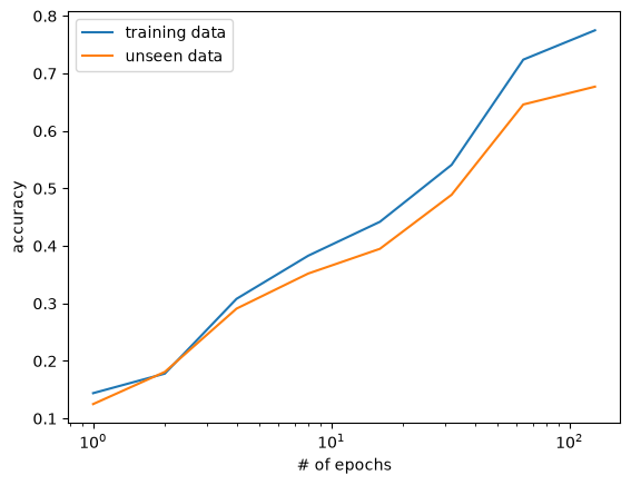
Increasing the number of epochs seems to help with both the training and unseen data.

Effect of the training sample size

Now let’s vary the size of the training sample

ntrain = [10, 30, 100, 300, 1000, 3000, 10000]
accuracy_trained = []
accuracy_unseen = []

for nt in ntrain:
    nn = NeuralNetwork(num_training_unique=nt,
                       hidden_layer_size=50, data_class=ModelDataCategorical)    
    nn.train(n_epochs=100)
    accuracy_trained.append(nn.check_accuracy())
    accuracy_unseen.append(nn.test_unseen())    

fig, ax = plt.subplots()

ax.plot(ntrain, accuracy_trained, label="training data")
ax.plot(ntrain, accuracy_unseen, label="unseed data")
ax.set_xscale("log")
ax.set_xlabel("# of training pairs")
ax.set_ylabel("accuracy")

Text(0, 0.5, 'accuracy')

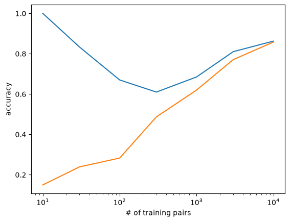
Here the number of training pairs helps most with the unseen data. This makes sense, because we have less of a chance of “memorizing” the training data if there is a lot of it.

Effect of hidden layer size

nhidden = [5, 10, 20, 50, 100, 200]
accuracy_trained = []
accuracy_unseen = []

for nh in nhidden:
    nn = NeuralNetwork(num_training_unique=1000,
                       hidden_layer_size=nh, data_class=ModelDataCategorical)    
    nn.train(n_epochs=100)
    accuracy_trained.append(nn.check_accuracy())
    accuracy_unseen.append(nn.test_unseen())    

fig, ax = plt.subplots()

ax.plot(nhidden, accuracy_trained, label="training data")
ax.plot(nhidden, accuracy_unseen, label="unseen data")
ax.set_xscale("log")
ax.set_xlabel("hidden layer size")
ax.set_ylabel("accuracy")
ax.legend()

<matplotlib.legend.Legend at 0x7f7e3206d030>

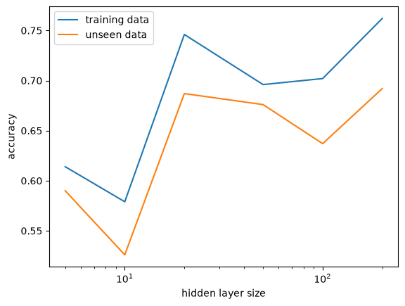
The size of the hidden layer helps a bit, but it seems to saturate after a while.

By far the best improvement we can get for unseen data is to train it on a larger number of training data pairs. If we show it more variety, then it is not overconstraining to just the data that it has seen.

A final look

Let’s run the network one last time, with a large number of training pairs and a large hidden layer and try to understand what the trained matrices look like.

nn = NeuralNetwork(num_training_unique=5000,
                   hidden_layer_size=100, data_class=ModelDataCategorical)
nn.train(n_epochs=100)

nn.check_accuracy()

0.8994

nn.test_unseen()

0.873

Excluding the activation function, the action of the network is to do \({\bf A B x}\), so lets look at the matrix \({\bf A B}\)

fig, ax = plt.subplots()

im = ax.imshow(nn.A @ nn.B)
fig.colorbar(im, ax=ax)

<matplotlib.colorbar.Colorbar at 0x7f7e31e9fd00>

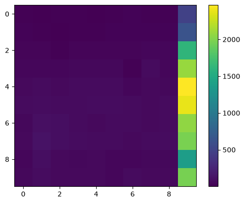
Notice that all of the large elements are in the last column—that is what “sees” the last element in the input vector \({\bf x}\).