Burgers’ Equation

The inviscid Burgers’ equation is the simplest nonlinear wave equation, and serves as a great stepping-stone toward doing full hydrodynamics.

\[u_t + u u_x = 0\]

This looks like the linear advection equation, except the quantity being advected is the velocity itself. This means that \(u\) is no longer a constant, but can vary in space and time.

Written in conservative form,

\[\frac{\partial u}{\partial t} + \frac{\partial F(u)}{\partial x} = 0\]

it appears as:

\[u_t + \left [ \frac{1}{2} u^2 \right ]_x = 0\]

so the flux is \(F(u) = \frac{1}{2} u^2\).

In the finite volume approach, we integrate over the volume of a cell to get the update:

\[\frac{\partial \langle u \rangle_i}{\partial t} = - \frac{1}{\Delta x} (F_{i+1/2} - F_{i-1/2})\]

To second order accuracy, as we saw previously, \(\langle u \rangle_i \approx u_i\), so we’ll drop the \(\langle \rangle\) here.

Nonlinear behavior

Our solution method is essentially the same, aside from the Riemann problem. We still want to use the idea of upwinding, but now we have a problem—the nonlinear nature of the Burgers’ equation means that information can “pile up” and we lose track of where the flow is coming from. This gives rise to a nonlinear wave called a shock.

For the linear advection equation, the solution was unchanged along the lines \(x - ut = \mbox{constant}\)—we called these the characteristic curves.

We can visualize the characteristics as show below:

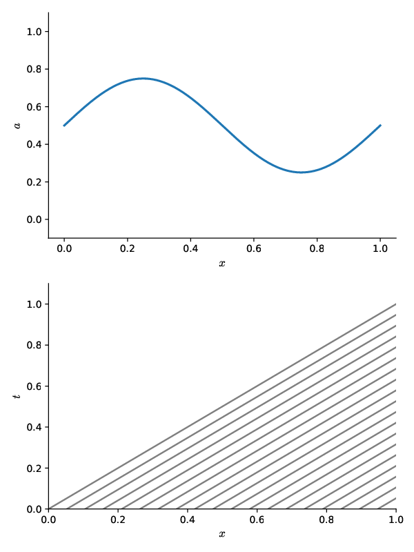
Fig. 5 The initial \(a(x, t=0)\) state (top) and the characteristic curves in the \(x\)-\(t\) spacetime diagram (bottom). We see that at any \(t > 0\), we find the value of \(a(x, t)\) by simply tracing backwards along the characteristic curve to the initial conditions. Since \(u\) is constant in the advection equation, the characteristic curves are parallel.

The characteristic curves are the curves on which the solution is constant. For Burgers’ equation, the characteristic curves are given by \(dx/dt = u\), but now \(u\) varies in the domain. To see this, look at the change of \(u\) in a fluid element (the full, or Lagrangian time derivative):

\[\frac{du}{dt} = \frac{\partial u}{\partial t} + \frac{dx}{dt} \frac{\partial u}{\partial x} = \frac{\partial u}{\partial t} + u \frac{\partial u}{\partial x} = 0\]

We see that \(du/dt = 0\) since it just gives us the Burgers equation. So \(u\) is constant along the curves \(dx/dt = u\), but now \(u\) varies in the domain. So if we look at the characteristic curves in the spacetime diagram, we get:

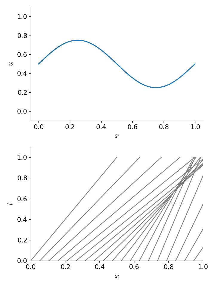
Fig. 6 Converging characteristic curves for Burgers’s equation resulting from an initially non-uniform velocity.

Now we see that, for these initial conditions, at some point in the future the characteristics intersect. This means that there is not a unique curve that we can trace back along to find the value of \(u(x,t)\). The information about where the solution was coming from was lost. This is the situation of a shock. The correct solution here is to put a discontinuous jump between the left and right states where the characteristics intersect. The speed of the shock can be found from the Rankine-Hugoniot conditions.

It is also possible to get a rarefaction if the characteristics diverge:

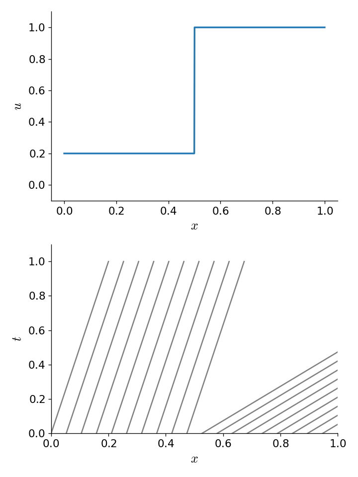
Fig. 7 Diverging characteristics resulting from an initially non-uniform velocity