FFT Review: Cleaning a Signal

Consider the following data:

signal.txt

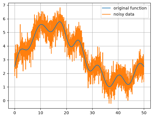
This contains data of a function polluted with noise. We want to remove the noise to recover the original function. The three columns in the file are: \(t\), \(f^\mathrm{(orig)}(t)\), and \(f^\mathrm{(noisy)}(t)\).

import numpy as np
import matplotlib.pyplot as plt

data = np.loadtxt("signal.txt")

fig, ax = plt.subplots()
ax.plot(data[:, 0], data[:, 1], label="original function", zorder=100)
ax.plot(data[:, 0], data[:, 2], label="noisy data")
ax.grid()
ax.legend()

<matplotlib.legend.Legend at 0x7f1908118850>

We will clean this by convolving the noisy data with a Gaussian.

A convolution is defined as:

\[(f \star g)(t) \equiv \int_{-\infty}^{\infty} f(\tau) g(t - \tau) d\tau\]

It is easy to compute this with FFTs, via the convolution theorem:

\[\mathcal{F}\{f \star g\} = \mathcal{F}\{f\} \, \mathcal{F}\{g\}\]

Here \(\mathcal{F}\{\}\) indicates taking the Fourier transform. That is the Fourier transform of the convolution of \(f\) and \(g\) is simply the product of the individual transforms of \(f\) and \(g\). This allows us to compute the convolution via multiplication in Fourier space and then take the inverse transform, \(\mathcal{F}^{-1}\{\}\), to recover the convolution in real space:

\[f \star g = \mathcal{F}^{-1}\{ \mathcal{F}\{f\} \, \mathcal{F}\{g\}\}\]

Let’s consider our function \(g(t)\) to be a Gaussian (we’ll call this the kernel):

\[g(t) = \frac{1}{\sigma \sqrt{2 \pi}}\, e^{-\frac{1}{2} (t/\sigma)^2}\]

Important

This kernel is normalized such that the integral under it is 1. This ensures that we don’t introduce a vertical shift in the data when we convolve.

We want to do the following:

• Make the kernel periodic on the domain defined by the \(t\) in the signal.txt file.

  Tip

  You can do this simply by left-right flipping the definitions above and applying them at the far end of the domain.

  Important

  Make sure that your kernel function is normalized by ensuring that it sums to \(1\) on the domain. You might need to sum up the values and divide by the sum.

• Take the FFT (or DFT) of \(f^\mathrm{(noisy)}(t)\) and the FFT of the kernel and plot them.

• Compute the convolution of \(f^\mathrm{(noisy)}(t)\) and \(g(x)\) in Fourier space and transform back to real space, and plot the de-noised function together with the original signal from the signal.txt (i.e., \(f^\mathrm{(orig)}(t)\)).

• Experiment with the tunable parameter, \(\sigma\), to see how clean you can get the noisy data and comment on what you see.

t = data[:, 0]
original = data[:, 1]
signal = data[:, 2]

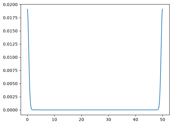
Let’s define our Gaussian function. We want it centered at \(t = 0\), but we also need it to be periodic in the domain, so we will flip it and sum and normalize:

def gaussian(t, sigma=0.5):
    """ a gaussian kernel """

    g = 1.0/(sigma*np.sqrt(2.0*np.pi))*np.exp(-0.5*(t/sigma)**2)
    g = g[:] + g[::-1]
    gsum = np.sum(g)
    return g/gsum

kernel = gaussian(t)

fig, ax = plt.subplots()
ax.plot(t, kernel)

[<matplotlib.lines.Line2D at 0x7f190801b7d0>]

Now let’s take the FFT of our signal and kernel

Next compute the convolution in frequency space

conv = fft_signal * fft_kernel

---------------------------------------------------------------------------
NameError                                 Traceback (most recent call last)
Cell In[8], line 1
----> 1 conv = fft_signal * fft_kernel

NameError: name 'fft_signal' is not defined

Finally convert back to real space—note we only care about the real part

Let’s plot the smoothed signal and the original to see how we did

Note

This process is used a lot in image processing both to remove noise and to compensate for the behavior of cameras to sharpen images. In image processing programs, this is what is done in the Gaussian blur transform.