
Application: Degenerate Electrons#
In white dwarfs, electron degeneracy pressure provides the dominant support against gravity. Electrons are fermions, and when the density of the star is high, they are packed closely together. Quantum mechanical effects come into play, and the electrons no longer behave as an ideal gas, but instead exhibit large pressure even at very low (or zero) temperature.
The origin of this is Fermi-Dirac statistics—no two electrons can occupy the same state, so as they get confined to a smaller and smaller volume, they need to take on larger momenta.
The distribution function describes the properties of the electrons, and has the following meaning: \(n(p) d^3 x d^3 p\) is the number of particles with momentum \(p\) in a volume \(d^3x\). Our distribution function is:
where \(\mathcal{E}\) is the kinetic energy of the electron, \(T\) is the temperature, and \(\Psi\) is the degeneracy parameter which is related to the chemical potential, \(\mu\), and the Fermi energy, \(\mathcal{E}_F\), as:
Note
Some sources use \(\eta\) instead of \(\Psi\) for the degeneracy parameter.
The electrons are degenerate when \(\Psi \gg 1\), which means that the Fermi energy is much greater than the thermal energy. The electrons behave as an ideal gas when \(-\Psi \gg 1\) (in this case, the \(+1\) in the denominator of \(n(p)\) is insignificant and we get the Maxwell-Boltzmann distribution).
To get the number density, we integrate over all momenta:
The pressure and specific internal energy, \(e\), are then found as:
Behavior of distribution function with \(\Psi\)#
Let’s look at the behavior of the distribution function. Consider:
let’s define
then we have
and for each choice of \(\Psi\) we have a unique distribution.
We note that \(\xi/\Psi = \mathcal{E}/\mathcal{E}_F\).
import numpy as np
import matplotlib.pyplot as plt
def F(xi, psi=100):
    return 1.0 / (np.exp(xi - psi) + 1)
Let’s look at the case of \(\Psi > 1\)
fig, ax = plt.subplots()

# we'll work in terms of r = xi / Psi
r = np.linspace(0, 4, 200)

for psi in [1, 2, 10, 20, 100]:
    ax.plot(r, F(psi * r, psi=psi), label=f"$\Psi = {psi}$")

ax.legend()
ax.set_ylabel("$F$")
ax.set_xlabel(r"$\mathcal{E}/\mathcal{E}_F$")
<>:7: SyntaxWarning: "\P" is an invalid escape sequence. Such sequences will not work in the future. Did you mean "\\P"? A raw string is also an option.
<>:7: SyntaxWarning: "\P" is an invalid escape sequence. Such sequences will not work in the future. Did you mean "\\P"? A raw string is also an option.
/tmp/ipykernel_3800/289879296.py:7: SyntaxWarning: "\P" is an invalid escape sequence. Such sequences will not work in the future. Did you mean "\\P"? A raw string is also an option.
  ax.plot(r, F(psi * r, psi=psi), label=f"$\Psi = {psi}$")
Text(0.5, 0, '$\\mathcal{E}/\\mathcal{E}_F$')
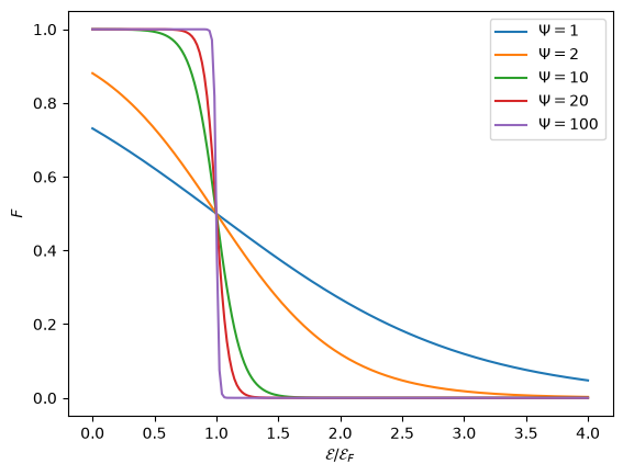
As we see, as \(\Psi \rightarrow \infty\), the distribution, \(F(\mathcal{E})\) becomes a step function. This is the limit of complete degeneracy, and we have:
We can alternately use the Fermi momentum, \(p_F\) to describe the location of the step.
With this form, the integral for number density is trivial:
where we switched to spherical coordinates in momentum space: \(d^3p \rightarrow 4\pi p^2 dp\).
For other values of \(\Psi\), we have a problem:
We don’t know what the value of \(\Psi\) is ahead of time. Instead, we typically know what the density of the star is, and we can find the number density of electrons as:
where \(Y_e\) is the electron fraction (typically around \(1/2\) for compositions heavier than hydrogen). This means that given \(\rho, T\), we can solve for \(\Psi\).
Once we have \(\Psi\), we can then find the pressure and energy of the gas.
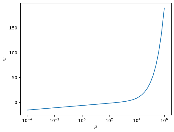
Finding the trend of \(\Psi\) with \(\rho, T\)#
Let’s now implement an algorithm to find the \(\Psi\) that corresponds to an input \(\rho\) (or \(n_e\)) and \(T\).
We first need a function to compute \(n_e\) given a \(T\) and a guess for \(\Psi\). We’ll use our composite Simpson’s integration for this.
We’ll assume that we are non-relativistic, so
Note
For \(\rho > 10^6~\mathrm{g~cm^{-3}}\) relativistic effects are important, and we would need to use a more general form for \(\mathcal{E}(p)\).
Our integral is then:
We can make a change of variables:
and then we have:
Note
Traditionally we express things in terms of \(\mathcal{E}\), so that means:
and
and then we have:
Then making it dimensionless using:
we get:
Integrals of the form:
are called Fermi-Dirac integrals. We can write our number density as:
There are a lot of papers that seek approximations to this type of integral, since they come up so often when dealing with degenerate matter.
Caution
Integrating \(F_n(\Psi)\) using Simpson’s rule for \(n = \pm 1/2\) is difficult because there are singularities in the derivatives at the origin. See Cloutman 1989 for a discussion.
We’ll stick with working with our dimensionless momentum, \(x\).
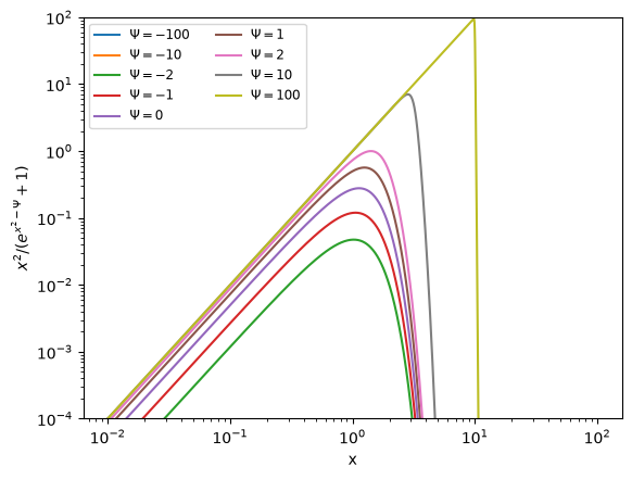
Let’s write a function that returns the integrand
def integrand(x, psi):
    return x**2 / (np.exp(x**2 - psi) + 1.0)
and now lets plot this for various \(\Psi\)
fig, ax = plt.subplots()
x = np.linspace(0, 100, 10000)
for psi in [-100, -10, -2, -1, 0, 1, 2, 10, 100]:
    ax.plot(x, integrand(x, psi), label=rf"$\Psi = {psi}$")

ax.legend(fontsize="small", ncol=2)

ax.set_xscale("log")
ax.set_yscale("log")

ax.set_xlabel("x")
ax.set_ylabel(r"$x^2 / (e^{x^2-\Psi} + 1)$")

ax.set_ylim(1.e-4, 1.e2)
/tmp/ipykernel_3800/3209928939.py:2: RuntimeWarning: overflow encountered in exp
  return x**2 / (np.exp(x**2 - psi) + 1.0)
(0.0001, 100.0)
Now let’s try scaling the integrand into \([0, 1]\). We’ll use the same technique we did for integrating the Planck function.
SMALL = 1.e-30

def zv(x, alpha):
    """ transform the variable x -> z """
    return x/(alpha + x)

def xv(z, alpha):
    """ transform back from z -> x """
    return alpha*z/(1.0 - z + SMALL)
fig, ax = plt.subplots()

z = np.linspace(0, 1, 100)
alpha = 2.0

x = np.linspace(0, 100, 10000)
for psi in [-100, -10, -2, -1, 0, 1, 2, 10, 100]:
    ax.plot(z, integrand(xv(z, alpha), psi), label=rf"$\Psi = {psi}$")

ax.legend(fontsize="small", ncol=2)
ax.set_yscale("log")

ax.set_xlabel("z")
ax.set_ylabel(r"$x(z)^2 / (e^{x(z)^2-\Psi} + 1)$")

ax.set_ylim(1.e-10, 100)
/tmp/ipykernel_3800/3209928939.py:2: RuntimeWarning: overflow encountered in exp
  return x**2 / (np.exp(x**2 - psi) + 1.0)
(1e-10, 100)
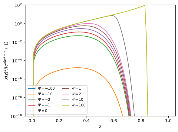
This looks reasonable. We might need to worry about resolving the sharp drop for the very large \(\Psi\) (when we are completely degenerate). But we’ll produce an estimate of the error in the integral as we compute it.
First the fundamental constants we need
# CGS constants

h_planck = 6.63e-27
k_B = 1.38e-16
m_e = 9.11e-28
m_u = 1.67e-24
Now a Simpson’s rule integrator for computing our integral, using the techniques we developed earlier for integrating to infinity.
def fd_integral(N, psi):
    """compute the integral over the Fermi-Dirac distribution
    using Simpsons rule with N intervals"""

    assert N % 2 == 0

    # we will transform from integrating over x to integrating over
    # z = x / (c + x) with z = [0, 1]

    alpha = 2.0
    z = np.linspace(0.0, 1.0, N+1, endpoint=True)

    I = 0.0
    for n in range(0, N, 2):
        fl = integrand(xv(z[n], alpha), psi) / (1.0 - z[n] + SMALL)**2
        fc = integrand(xv(z[n+1], alpha), psi) / (1.0 - z[n+1] + SMALL)**2
        fr = integrand(xv(z[n+2], alpha), psi) / (1.0 - z[n+2] + SMALL)**2

        I += (1.0/3.0) * (z[n+1] - z[n]) * (fl + 4*fc + fr)

    I *= alpha
    return I
Warning
Our integration does nothing to ensure that the number of bins, \(N\), is reasonable. Ideally, we want some sort of error estimation when we do our integration. We can do this crudely by integrating with \(N\) and then \(2N\) bins and computing the relative change in \(I\). We’ll do this below.
Now a function that returns \(n_e\). This does the integral, ensuring we meet some accuracy, and adds in the physical constants to give us \(n_e\).
def compute_ne(T, psi, N=100, tol=1.e-8):
    """given a temperature and degeneracy parameter, psi,
    compute the number density of electrons by integrating
    the Fermi-Dirac distribution over all momenta"""

    # we'll do the dimensionless integral of
    # x**2 / (exp(x**2 - psi) + 1) using Simpson's rule
    # we will pick a value of N and do the integration
    # and then change N until the error is small

    err = 1.e30
    I_old = 1.e30

    while err > tol:
        I = fd_integral(N, psi)
        err = np.abs(I - I_old) / np.abs(I_old)
        I_old = I

        N *= 2

    ne = 8.0 * np.pi / h_planck**3 * (2.0 * m_e * k_B * T)**1.5 * I
    return ne
Now we want to do a root find on this. We will start with bisection, although we note that there are better methods we could do.
def find_psi(rho, T, Ye=0.5, tol=1.e-6):
    """given rho, T, we want to find the degeneracy parameter, psi"""

    ne_input = rho * Ye / m_u

    psi_low = -100
    psi_high = 1000

    # we want to zero ne(T, psi) - ne_input)

    ne_low = compute_ne(T, psi_low) - ne_input
    ne_high = compute_ne(T, psi_high) - ne_input

    if ne_low * ne_high > 0:
        print("no root in this interval")

        return None

    err = 1.e10
    psi_mid = 0.5 * (psi_low * psi_high)

    while err > tol:
        ne_mid = compute_ne(T, psi_mid) - ne_input

        if ne_low * ne_mid > 0:
            # the root is in the right half of the interval
            psi_low = psi_mid
            ne_low = ne_mid
        else:
            psi_high = psi_mid
            ne_high = ne_mid

        psi_mid = 0.5 * (psi_low + psi_high)
        err = np.abs(psi_low - psi_high) / np.abs(psi_mid)

    return psi_mid
This is an implementation of the secant method which is essentially Newton’s method with the derivative computed via a finite difference.
def find_psi2(rho, T, Ye=0.5, tol=1.e-6):
    """given rho, T, we want to find the degeneracy parameter, psi"""

    ne_input = rho * Ye / m_u

    psi_m1 = 10
    psi_0 = 20

    # we want to zero ne(T, psi) - ne_input)

    ne_m1 = compute_ne(T, psi_m1) - ne_input

    err = 1.e10

    while err > tol:
        ne_0 = compute_ne(T, psi_0) - ne_input
        dne_dpsi = (ne_0 - ne_m1) / (psi_0 - psi_m1)

        psi_m1 = psi_0
        ne_m1 = ne_0

        psi_0 -= ne_0 / dne_dpsi

        err = np.abs(ne_0 / dne_dpsi) / np.abs(psi_0)

    return psi_0
T = 1.e7
rhos = np.logspace(-4, 6, 50)
psis = []

for rho in rhos:
    psi = find_psi2(rho, T)
    psis.append(psi)
/tmp/ipykernel_3800/3209928939.py:2: RuntimeWarning: overflow encountered in exp
  return x**2 / (np.exp(x**2 - psi) + 1.0)
fig, ax = plt.subplots()
ax.plot(rhos, psis)
ax.set_xlabel(r"$\rho$")
ax.set_ylabel(r"$\Psi$")
ax.set_xscale("log")
C++ implementation#
A C++ version of the above method is available as degeneracy.cpp
// Given an electron number density, n_e, integrate the Fermi-Dirac
// distribution and find the degeneracy parameter that gives that
// number density.
//
// We assume that we are non-relativisitic and work in terms
// of dimensionless momentum, x = p / (m_e c).
//
// We are ultimately integrating
//
// n_e = (8π/h^3) (2m_e k T)^(3/2) ∫ x^2 dx / (exp(x^2 - psi) + 1)
//
// where psi is the degeneracy parameter.

#include <iostream>
#include <cmath>
#include <cassert>
#include <limits>

namespace {
    constexpr double SMALL{1.e-30};
    constexpr double h_planck{6.63e-27};
    constexpr double k_B{1.38e-16};
    constexpr double m_e{9.11e-28};
    constexpr double m_u {1.67e-24};
}

inline
double integrand(const double x, const double psi) {
    return x * x / (std::exp(x*x - psi) + 1.0);
}

inline
double xv(const double z, const double alpha) {
    return alpha * z / (1.0 - z + SMALL);
}

inline
double fd_integral(const int N, const double psi) {

    assert(N % 2 == 0);

    // we will transform from integrating over x to integrating over
    // z = x / (alpha + x) with z = [0, 1]

    double alpha{2.0};

    // N is the number of intervals
    double dz = 1.0 / static_cast<double>(N);

    double I{0.0};
    for (int n = 0; n < N; n += 2) {
        double zl{n * dz};
        double zc{(n + 1) * dz};
        double zr{(n + 2) * dz};

        double fl = integrand(xv(zl, alpha), psi) / std::pow(1.0 - zl + SMALL, 2);
        double fc = integrand(xv(zc, alpha), psi) / std::pow(1.0 - zc + SMALL, 2);
        double fr = integrand(xv(zr, alpha), psi) / std::pow(1.0 - zr + SMALL, 2);

        I += (1.0/3.0) * dz * (fl + 4*fc + fr);
    }
    I *= alpha;
    return I;
}

inline
double compute_ne(const double T, const double psi,
                  double tol=1.e-8) {
    // given a temperature and degeneracy parameter, psi, compute the
    // number density of electrons by integrating the Fermi-Dirac
    // distribution over all momenta

    // we'll do the dimensionless integral of
    // x**2 / (exp(x**2 - psi) + 1) using Simpson's rule
    // we will pick a value of N and do the integration
    // and then change N until the error is small

    // we'll start with N = 50 and then keep doubling
    // until the difference in I is small

    int N{50};
    double err = std::numeric_limits<double>::max();
    double I_old = std::numeric_limits<double>::max();

    double I{};

    while (err > tol) {
        I = fd_integral(N, psi);
        err = std::abs(I - I_old) / std::abs(I_old);
        I_old = I;
        N *= 2;
    }

    double ne = 8.0 * M_PI / std::pow(h_planck, 3) *
        std::pow(2.0 * m_e * k_B * T, 1.5) * I;

    return ne;
}

inline
double find_psi(const double rho, const double T, const double Ye,
                double tol=1.e-6) {
    // use a secant method to find the psi that gives the correct
    // n_e / density (rho)

    double ne_input = rho * Ye / m_u;

    // initial guesses
    double psi_m1{10.0};
    double psi_0{20.0};

    // we want to zero ne(T, psi) - ne_input

    auto ne_m1 = compute_ne(T, psi_m1) - ne_input;

    double err = std::numeric_limits<double>::max();

    while (err > tol) {
        auto ne_0 = compute_ne(T, psi_0) - ne_input;
        double dne_dpsi = (ne_0 - ne_m1) / (psi_0 - psi_m1);

        psi_m1 = psi_0;
        ne_m1 = ne_0;

        psi_0 -= ne_0 / dne_dpsi;

        err = std::abs(ne_0 / dne_dpsi) / std::abs(psi_0);
    }

    return psi_0;
}

int main() {

    double T{1.e7};
    double Ye = 0.5;

    double rho_min{1.e-4};
    double rho_max{1.e6};

    int N{50};

    double dlogrho = (std::log10(rho_max) - std::log10(rho_min)) /
        static_cast<double>(N - 1);

    for (int nrho = 0; nrho < N; ++nrho) {
        double rho = std::pow(10.0, std::log10(rho_min) + nrho*dlogrho);

        auto psi = find_psi(rho, T, Ye);
        std::cout << rho << " " << psi << std::endl;
    }
}
Improvements#
Simpson’s rule is not the best method for integrating this. In particular, we see that for \(\Psi \gg 1\), we need a lot of points because of the sharp step in the distribution function. A better method would be to not use uniform intervals when doing this integral.
For example, scipy.integrate.quad uses the QUADPACK library to do the integration, and uses a Gaussian quadrature for constructing the integral.
The secant method begins with an initial guess, and we could try to seed the initial guess for \(\Psi\) with the guess from the previous \(\rho\) solution. This would accelerate convergence.
Physically, we should extend \(\mathcal{E}(p)\) to be relativistic, which would allow us to probe higher densities.
SciPy implementation#
Here’s a version using the integration and root finding functions available in SciPy
from scipy import integrate, optimize
def ne_scipy(T, psi):
    I, err = integrate.quad(integrand, 0, np.inf, args=(psi))
    ne = 8.0 * np.pi / h_planck**3 * (2.0 * m_e * k_B * T)**1.5 * I
    return ne

def find_psi_scipy(rho, T, Ye=0.5):

    ne_input = rho * Ye / m_u
    psi_low = -100
    psi_high = 1000

    psi = optimize.brentq(lambda psi: ne_input - ne_scipy(T, psi), psi_low, psi_high)
    return psi
T = 1.e7
rhos = np.logspace(-4, 6, 50)
psis = []

for rho in rhos:
    psi = find_psi_scipy(rho, T)
    psis.append(psi)

fig, ax = plt.subplots()
ax.plot(rhos, psis)
ax.set_xlabel(r"$\rho$")
ax.set_ylabel(r"$\Psi$")
ax.set_xscale("log")
/tmp/ipykernel_3800/3209928939.py:2: RuntimeWarning: overflow encountered in exp
  return x**2 / (np.exp(x**2 - psi) + 1.0)