
Two Grid Correction#
Before we do multigrid, we can understand the basic flow by using 2 grids: a fine and coarse grid.
We want to solve:
with suitable boundary conditions. Imagine that we have a approximate solution, \(\tilde{\phi}\), then we can define the error with respect to the true solution, \(\phi^{\mathrm{true}}\) as:
Our Poisson equation is linear, so we can apply the \(\nabla^2\) operator to our error:
This since \(\tilde{\phi}\) is just our approximation to \(\phi^{\mathrm{true}}\), this is just the residual, so:
Notice that this is the same type of equation as our original equation. But the boundary conditions are now homogeneous (of the same type as the original) regardless of whether they were inhomogeneous or homogeneous originally. For example:
If the BCs were inhomogeneous Dirichlet, \(\phi(a) = A\), then
\[e(a) = \phi^{\mathrm{true}}(a) - \tilde{\phi}(a) = 0\]since both the true solution and our approximation satisfy the same boundary conditions.
Likewise, if the BCs were inhomogeneous Neumann, \(\phi^\prime(a) = C\), then
\[e^{\prime}(a) = \phi^{\mathrm{true},\prime}(a) - \tilde{\phi}^{\prime}(a) = 0\]
The key idea in multigrid is that long wavelength errors take longer to smooth away. But long wavelength errors look shorter wavelength on a coarser grid. This suggests that we smooth a bit on a fine grid to get rid of the short wavelength errors and then transfer down to a coarser grid, and smooth the error equation there, and then bring the error back to the fine grid to correct the fine grid solution.
We’ll use the superscript \(h\) to represent the fine grid and the superscript \(2h\) to represent a grid that is coarser by a factor of 2.
Here’s the basic flow:
Smooth for \(N_\mathrm{smooth}\) iterations on the fine grid, solving \(\nabla^2 \phi = f\) to get an approximation \(\tilde{\phi}\)
Compute the residual, on the fine grid:
\[r^h = f - \nabla^2 \tilde{\phi}\]Restrict \(r^h\) to the coarse grid:
\[r^{2h} \leftarrow r^h\]Solve the error equation on the coarse grid:
\[\nabla^2 e^{2h} = r^{2h}\]Prolong the error from the coarse grid up to the fine grid:
\[e^{2h} \rightarrow e^{h}\]Correct the fine grid solution, since by the definition of \(e\), \(\phi^{\mathrm{true}} = \tilde{\phi} + e\)
\[\tilde{\phi}^h \leftarrow \tilde{\phi}^h + e^h\]This correction may have introduced some short wavelength noise (from the prolongation), so smooth \(\nabla^2 \phi = f\) on the fine grid for \(N_\mathrm{smooth}\) iterations.
For now, to solve the error equation, we’ll resort to simply smoothing until all of residual is below our desired tolerance. In a little bit though, we’ll see that we can just do this procedure recursively for that step.
import numpy as np
We’ll start with a grid class that has storage for the solution, righthand side, and residual, and knows how to fill boundary conditions, prolong, and restrict the data, and take a norm.
We write the restriction and prologation routines to take an argument that is the data we wish to operate on.
We also provide a residual routine that works on the data and stores the residual as grid data.
We store the solution variable (\(\phi\) or \(e\)) as Grid.v in this class.
import grid
%cat grid.py
import numpy as np


class Grid:

    def __init__(self, nx, ng=1, xmin=0, xmax=1,
                 bc_left_type="dirichlet", bc_left_val=0.0,
                 bc_right_type="dirichlet", bc_right_val=0.0):

        self.xmin = xmin
        self.xmax = xmax
        self.ng = ng
        self.nx = nx

        self.bc_left_type = bc_left_type
        self.bc_left_val = bc_left_val

        self.bc_right_type = bc_right_type
        self.bc_right_val = bc_right_val

        # python is zero-based.  Make easy integers to know where the
        # real data lives
        self.ilo = ng
        self.ihi = ng+nx-1

        # physical coords -- cell-centered
        self.dx = (xmax - xmin)/(nx)
        self.x = xmin + (np.arange(nx+2*ng)-ng+0.5)*self.dx

        # storage for the solution
        self.v = self.scratch_array()
        self.f = self.scratch_array()
        self.r = self.scratch_array()

    def scratch_array(self):
        """return a scratch array dimensioned for our grid """
        return np.zeros((self.nx+2*self.ng), dtype=np.float64)

    def norm(self, e):
        """compute the L2 norm of e that lives on our grid"""
        return np.sqrt(self.dx * np.sum(e[self.ilo:self.ihi+1]**2))

    def compute_residual(self):
        """compute and return the residual"""

        self.r[self.ilo:self.ihi+1] = self.f[self.ilo:self.ihi+1] - \
            (self.v[self.ilo+1:self.ihi+2] -
             2 * self.v[self.ilo:self.ihi+1] +
             self.v[self.ilo-1:self.ihi]) / self.dx**2

    def fill_bcs(self):
        """fill the boundary conditions on phi"""

        # we only deal with a single ghost cell here

        # left
        if self.bc_left_type.lower() == "dirichlet":
            self.v[self.ilo-1] = 2 * self.bc_left_val - self.v[self.ilo]
        elif self.bc_left_type.lower() == "neumann":
            self.v[self.ilo-1] = self.v[self.ilo] - self.dx * self.bc_left_val
        else:
            raise ValueError("invalid bc_left_type")

        # right
        if self.bc_right_type.lower() == "dirichlet":
            self.v[self.ihi+1] = 2 * self.bc_right_val - self.v[self.ihi]
        elif self.bc_right_type.lower() == "neumann":
            self.v[self.ihi+1] = self.v[self.ihi] - self.dx * self.bc_right_val
        else:
            raise ValueError("invalid bc_right_type")

    def restrict(self, a):
        """restrict the data to a coarser (by 2x) grid"""

        assert len(a) == self.nx + 2 * self.ng

        # create a coarse array
        ng = self.ng
        nc = self.nx//2

        ilo_c = ng
        ihi_c = ng + nc - 1

        coarse_data = np.zeros((nc + 2*ng), dtype=np.float64)

        coarse_data[ilo_c:ihi_c+1] = 0.5 * (a[self.ilo:self.ihi+1:2] +
                                            a[self.ilo+1:self.ihi+1:2])

        return coarse_data

    def prolong(self, a):
        """prolong the data in the current (coarse) grid to a finer (factor
        of 2 finer) grid using linear reconstruction.

        """

        assert len(a) == self.nx + 2 * self.ng

        # allocate an array for the coarsely gridded data
        ng = self.ng
        nf = self.nx * 2

        fine_data = np.zeros((nf + 2*ng), dtype=np.float64)

        ilo_f = ng
        ihi_f = ng + nf - 1

        # slopes for the coarse data
        m_x = self.scratch_array()
        m_x[self.ilo:self.ihi+1] = 0.5 * (a[self.ilo+1:self.ihi+2] -
                                          a[self.ilo-1:self.ihi])

        # fill the '1' children
        fine_data[ilo_f:ihi_f+1:2] = \
            a[self.ilo:self.ihi+1] - 0.25 * m_x[self.ilo:self.ihi+1]

        # fill the '2' children
        fine_data[ilo_f+1:ihi_f+1:2] = \
            a[self.ilo:self.ihi+1] + 0.25 * m_x[self.ilo:self.ihi+1]

        return fine_data
We also need the relax function we wrote previously. Here we just paste it below:
class TooManyIterations(Exception):
    pass

def relax(g, tol=1.e-8, max_iters=200000):

    iter = 0
    fnorm = g.norm(g.f)
    if fnorm == 0.0:
        fnorm = 1

    g.compute_residual()
    r = g.norm(g.r)

    while iter < max_iters and (tol is None or r > tol * fnorm):
        g.fill_bcs()

        g.v[g.ilo:g.ihi+1:2] = 0.5 * (-g.dx**2 * g.f[g.ilo:g.ihi+1:2] +
                                      g.v[g.ilo+1:g.ihi+2:2] +
                                      g.v[g.ilo-1:g.ihi:2])

        g.fill_bcs()

        g.v[g.ilo+1:g.ihi+1:2] = 0.5 * (-g.dx**2 * g.f[g.ilo+1:g.ihi+1:2] +
                                        g.v[g.ilo+2:g.ihi+2:2] +
                                        g.v[g.ilo:g.ihi:2])

        g.fill_bcs()

        g.compute_residual()
        r = g.norm(g.r)

        iter += 1

    if tol is not None and iter >= max_iters:
        raise TooManyIterations(f"too many iterations, niter = {iter}")
Now we can write our two-grid solver. We’ll solve the same system as before:
on \([0, 1]\) with homogeneous Dirichlet BCs.
def analytic(x):
    return -np.sin(x) + x * np.sin(1.0)

def f(x):
    return np.sin(x)
Here’s our implementation of the two grid solver
nx = 128
n_smooth = 10

# create the grids
fine = grid.Grid(nx)
coarse = grid.Grid(nx//2)

# initialize the RHS
fine.f[:] = f(fine.x)

# smooth on the fine grid
relax(fine, max_iters=n_smooth, tol=None)

# compute the residual
fine.compute_residual()

print("fine grid residual norm (after initial smoothing): ", fine.norm(fine.r))

# restrict the residual down to the coarse grid as the coarse rhs
coarse.f[:] = fine.restrict(fine.r)

# solve the coarse problem:
relax(coarse, tol=1.e-8)

coarse.compute_residual()
print("coarse grid residual norm (after smoothing): ", coarse.norm(coarse.r))

# prolong the error up from the coarse grid and correct the fine grid solution
fine.v += coarse.prolong(coarse.v)

fine.compute_residual()
print("fine grid residual norm (after prolongation): ", fine.norm(fine.r))

# smooth on the fine grid
relax(fine, max_iters=n_smooth, tol=None)

fine.compute_residual()
print("fine grid residual norm (after smoothing): ", fine.norm(fine.r))
fine grid residual norm (after initial smoothing): 0.7006172697956556
coarse grid residual norm (after smoothing):  4.9484569115558645e-09
fine grid residual norm (after prolongation):  1.8526271733335742
fine grid residual norm (after smoothing):  0.009477437263561143
Let’s look at the solution:
import matplotlib.pyplot as plt
fig = plt.figure()
ax = fig.add_subplot(211)

ax.plot(fine.x[fine.ilo:fine.ihi+1], fine.v[fine.ilo:fine.ihi+1])
ax.plot(fine.x[fine.ilo:fine.ihi+1], analytic(fine.x[fine.ilo:fine.ihi+1]), label="analytic", ls=":")

ax.set_ylabel(r"$\phi$")
ax.legend()

ax2 = fig.add_subplot(212)

e = fine.v - analytic(fine.x)
ax2.plot(fine.x[fine.ilo:fine.ihi+1], e[fine.ilo:fine.ihi+1])

ax2.set_xlabel("$x$")
ax2.set_ylabel("error")
Text(0, 0.5, 'error')
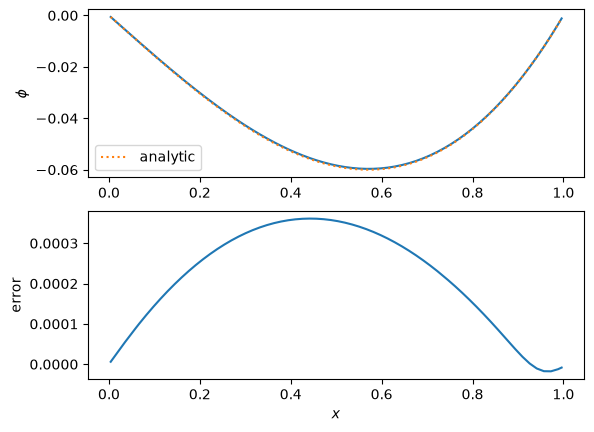
It seems odd that the residual on the fine grid after prolongation and smoothing is actually higher than it was before, but the error is all at short wavelengths now. To see this, simply comment out the final relax() call and look at the error plot above.