Second-order Euler solver#
import numpy as np
import matplotlib.pyplot as plt
We now have all the pieces needed to solve the Euler equation. The main difference with the Burgers’s are:
We are updating 3 variables, \(\rho, \rho u, \rho E\)
The Riemann problem is more complex
Our timestep constraint needs to consider the fastest wave
Our code will have essentially the same structure we used for advection and the Burgers’ solver:
Create our numerical grid
Set the initial conditions
Main timestep evolution loop
Compute the timestep
Loop to advance one step (count depends on the number of stages in the integrator)
Reconstruct the state to interfaces
Solve Riemann problem to find the fluxes through the interface
Do a conservative update of the state to the stage
Output
Grid and variables#
We’ll use the same finite-volume grid class we used with the earlier solvers.
The main information we need to setup the grid are the number of zones in the interior and the number of ghost cells.
To make life easier, we’ll have a simple class with indices that we use to index the fluid state arrays. We can pass this around and be sure that we are always accessing the correct fluid state.
class FluidVars:
    """A simple container that holds the integer indices we will use to
    refer to the different fluid components"""
    def __init__(self, gamma=1.4, C=0.8):
        self.nvar = 3

        # conserved variables
        self.urho = 0
        self.umx = 1
        self.uener = 2

        # primitive variables
        self.qrho = 0
        self.qu = 1
        self.qp = 2

        # EOS gamma
        self.gamma = gamma

        # CFL number
        self.C = C
This is the main class for managing the finite-volume grid. In addition to holding coordinate information and knowing the bounds of the domain, it also can fill the ghost cells and give you a scratch array that lives on the same grid.
Note that we now consider the state array to be 2-dimensional, with the second dimension the component.
class FVGrid:
    """The main finite-volume grid class for holding our fluid state."""

    def __init__(self, nx, ng, xmin=0.0, xmax=1.0, vars=None):

        self.xmin = xmin
        self.xmax = xmax
        self.ng = ng
        self.nx = nx

        self.lo = ng
        self.hi = ng+nx-1

        # physical coords -- cell-centered
        self.dx = (xmax - xmin)/(nx)
        self.x = xmin + (np.arange(nx+2*ng)-ng+0.5)*self.dx

        self.v = vars

    def scratch_array(self, nc=1):
        """ return a scratch array dimensioned for our grid """
        return np.squeeze(np.zeros((self.nx+2*self.ng, nc), dtype=np.float64))

    def fill_BCs(self, atmp):
        """ fill all ghost cells with zero-gradient boundary conditions """
        if atmp.ndim == 2:
            for n in range(atmp.shape[-1]):
                atmp[0:self.lo, n] = atmp[self.lo, n]
                atmp[self.hi+1:, n] = atmp[self.hi, n]
        else:
            atmp[0:self.lo] = atmp[self.lo]
            atmp[self.hi+1:] = atmp[self.hi]
Reconstruction#
We need to use the cell-averages to figure out what the fluid state is on the interfaces. We’ll reconstruct the cell-averages as piecewise lines that give us the same average in the zone. We then follow these lines to the interfaces to define the left and right state at each interface.
Usually we work in terms of the primitive variables, \({\bf q} = (\rho, u, p)\). So we first write a routine to do the algebraic transformation from conservative to primitive variables:
def cons_to_prim(g, U):
    """take a conservative state U and return the corresponding primitive
    variable state as a new array."""
    q = g.scratch_array(nc=g.v.nvar)

    q[:, g.v.qrho] = U[:, g.v.urho]
    q[:, g.v.qu] = U[:, g.v.umx]/U[:, g.v.urho]
    rhoe = U[:, g.v.uener] - 0.5*q[:, g.v.qrho]*q[:, g.v.qu]**2
    q[:, g.v.qp] = rhoe*(g.v.gamma - 1.0)

    return q
Next we need a routine to create the interface states. We’ll do this the same way as we did with Burgers’: construct a slope for each zone, \(\Delta {\bf q}\) based on the average state in the neighboring zones and use that to find the left and right states at each interface.
We’ll continue to use the minmod limiter.
def states(g, U):

    q = cons_to_prim(g, U)

    # construct the slopes
    dq = g.scratch_array(nc=g.v.nvar)

    for n in range(g.v.nvar):
        dl = g.scratch_array()
        dr = g.scratch_array()

        dl[g.lo-1:g.hi+2] = q[g.lo-1:g.hi+2,n] - q[g.lo-2:g.hi+1,n]
        dr[g.lo-1:g.hi+2] = q[g.lo:g.hi+3,n] - q[g.lo-1:g.hi+2,n]

        # these where's do a minmod()
        d1 = np.where(np.fabs(dl) < np.fabs(dr), dl, dr)
        dq[:, n] = np.where(dl*dr > 0.0, d1, 0.0)

    # now make the states

    # left state on i - 1/2
    q_l = g.scratch_array(nc=g.v.nvar)
    q_l[g.lo:g.hi+2, :] = q[g.lo-1:g.hi+1, :] + 0.5*dq[g.lo-1:g.hi+1, :]

    # right state on i - 1/2
    q_r = g.scratch_array(nc=g.v.nvar)
    q_r[g.lo:g.hi+2, :] = q[g.lo:g.hi+2, :] - 0.5*dq[g.lo:g.hi+2, :]

    return q_l, q_r
Riemann problem and conservative update#
After doing our reconstruction, we are left with a left and right state on an interface. To find the unique fluid state on the interface, we solve a Riemann problem,
We’ll use the solver we developed in the previous notebooks.
One we have the interface state, we can compute the fluxes using this state:
def cons_flux(state, v):
    """ given an interface state, return the conservative flux"""
    flux = np.zeros((v.nvar), dtype=np.float64)

    flux[v.urho] = state.rho * state.u
    flux[v.umx] = flux[v.urho] * state.u + state.p
    flux[v.uener] = (0.5 * state.rho * state.u**2 +
                     state.p/(v.gamma - 1.0) + state.p) * state.u
    return flux
To keep things simple, the Riemann solver is in a module now that we import: riemann_exact.py.
import riemann_exact as re
For a method-of-lines approach, we want to just compute the righthand side, \(A = -\partial F/\partial x\). Then we will turn our PDE into an ODE for time:
This routine will take the conserved state, \(U\), construct the left and right states at all interfaces, solve the Riemann problem to get the unique state on the boundary, and then compute the advective term and return it.
def make_flux_divergence(g, U):

    # get the states
    q_l, q_r = states(g, U)

    # now solve the Riemann problem
    flux = g.scratch_array(nc=g.v.nvar)

    for i in range(g.lo, g.hi+2):
        sl = re.State(rho=q_l[i, g.v.qrho], u=q_l[i, g.v.qu], p=q_l[i, g.v.qp])
        sr = re.State(rho=q_r[i, g.v.qrho], u=q_r[i, g.v.qu], p=q_r[i, g.v.qp])
        rp = re.RiemannProblem(sl, sr, gamma=g.v.gamma)
        rp.find_star_state()
        q_int = rp.sample_solution()
        flux[i, :] = cons_flux(q_int, g.v)

    A = g.scratch_array(nc=g.v.nvar)
    for n in range(g.v.nvar):
        A[g.lo:g.hi+1, n] = (flux[g.lo:g.hi+1, n] -
                             flux[g.lo+1:g.hi+2, n]) / g.dx

    return A
Timestep#
For the hydro equations, the speeds at which information travels are \(u\) and \(u \pm c\), so we use the largest speed here to compute the timestep:
def timestep(g, U):

    # compute the sound speed
    q = cons_to_prim(g, U)
    c = g.scratch_array()
    c[g.lo:g.hi+1] = np.sqrt(g.v.gamma *
                             q[g.lo:g.hi+1, g.v.qp] /
                             q[g.lo:g.hi+1, g.v.qrho])

    dt = g.v.C * g.dx / (np.abs(q[g.lo:g.hi+1, g.v.qu]) +
                         c[g.lo:g.hi+1]).max()
    return dt
Main driver#
This is the main driver.
This does 2nd-order RK (or Euler’s method) for the integration, and requires that we compute the advection terms twice to advance the solution by \(\Delta t\). The update looks like:
def mol_solve(nx, C=0.8, tmax=1.0, init_cond=None):
    """Perform 2nd order MOL integration of the Euler equations.
    You need to pass in a function foo(grid) that returns the
    initial conserved fluid state."""

    v = FluidVars(C=C)

    grid = FVGrid(nx, 2, vars=v)

    U = init_cond(grid)

    t = 0.0

    while t < tmax:
        dt = timestep(grid, U)
        if t + dt > tmax:
            dt = tmax - t

        grid.fill_BCs(U)
        k1 = make_flux_divergence(grid, U)

        U_tmp = grid.scratch_array(nc=v.nvar)
        for n in range(v.nvar):
            U_tmp[:, n] = U[:, n] + 0.5 * dt * k1[:, n]

        grid.fill_BCs(U_tmp)
        k2 = make_flux_divergence(grid, U_tmp)

        for n in range(v.nvar):
            U[:, n] += dt * k2[:, n]

        t += dt

    return grid, U
Example: Sod’s problem#
The Sod problem is a standard test problem, consisting of a left and right state separated by an initial discontinuity. As time evolves, a rightward moving shock and contact and leftward moving rarefaction form. We’ve actually been looking at these initial conditions as we developed the Riemann solver.
One reason this problem is so popular is that you can find the exact solution (it’s just the Riemann problem) and compare the performance of your code to the exact solution.
For comparison, here’s a file with the exact solution: sod-exact.out
Note
The exact solution will depend on your choice of \(\gamma\). The file above uses
which is appropriate for our atmosphere (diatomic molecules).
def sod(g):

    U = g.scratch_array(nc=g.v.nvar)

    # setup initial conditions -- this is Sod's problem
    rho_l = 1.0
    u_l = 0.0
    p_l = 1.0
    rho_r = 0.125
    u_r = 0.0
    p_r = 0.1

    idx_l = g.x < 0.5
    idx_r = g.x >= 0.5

    U[idx_l, g.v.urho] = rho_l
    U[idx_l, g.v.umx] =  rho_l * u_l
    U[idx_l, g.v.uener] = p_l/(g.v.gamma - 1.0) + 0.5 * rho_l * u_l**2

    U[idx_r, g.v.urho] = rho_r
    U[idx_r, g.v.umx] =  rho_r * u_r
    U[idx_r, g.v.uener] = p_r/(g.v.gamma - 1.0) + 0.5 * rho_r * u_r**2

    return U
g, U = mol_solve(64, tmax=0.2, init_cond=sod)
Let’s read in the exact solution from a data file
sod_exact = np.genfromtxt("sod-exact.out", skip_header=2, names=True)
v = FluidVars()

q = cons_to_prim(g, U)
fig = plt.figure()

ax = fig.add_subplot(311)
ax.scatter(g.x, q[:,v.qrho], marker="x", color="C0")
ax.plot(sod_exact["x"], sod_exact["rho"], color="C1")
ax.set_ylabel(r"$\rho$")

ax = fig.add_subplot(312)
ax.scatter(g.x, q[:,v.qu], marker="x", color="C0")
ax.plot(sod_exact["x"], sod_exact["u"], color="C1")
ax.set_ylabel(r"$u$")

ax = fig.add_subplot(313)
ax.scatter(g.x, q[:,v.qp], marker="x", color="C0")
ax.plot(sod_exact["x"], sod_exact["p"], color="C1")
ax.set_ylabel(r"$p$")
ax.set_xlabel(r"$x$")

fig.set_size_inches((6, 10))
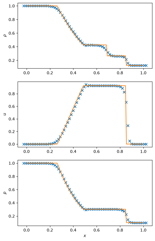
We see that we match the exact solution reasonably well. The contact discontinuity is smeared out a bit—that’s common, since velocity is constant across the contact, so it doesn’t self-steepen like a shock.
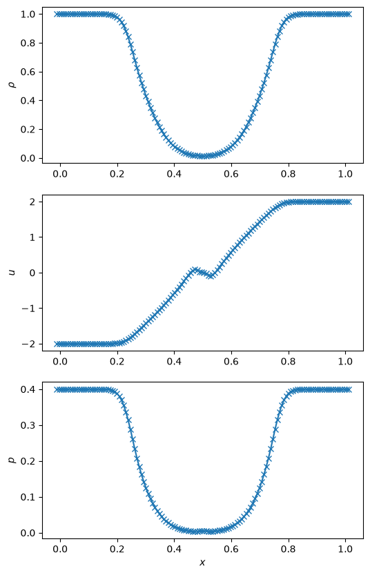
Example: double rarefaction#
Here’s a case where we have density and pressure constant but the velocity initially equal and opposite, resulting in a vacuum.
def double_rarefaction(g):

    U = g.scratch_array(nc=g.v.nvar)

    # setup initial conditions -- this is Sod's problem
    rho_l = 1.0
    u_l = -2.0
    p_l = 0.4
    rho_r = 1.0
    u_r = 2.0
    p_r = 0.4

    idx_l = g.x < 0.5
    idx_r = g.x >= 0.5

    U[idx_l, g.v.urho] = rho_l
    U[idx_l, g.v.umx] =  rho_l * u_l
    U[idx_l, g.v.uener] = p_l/(g.v.gamma - 1.0) + 0.5 * rho_l * u_l**2

    U[idx_r, g.v.urho] = rho_r
    U[idx_r, g.v.umx] =  rho_r * u_r
    U[idx_r, g.v.uener] = p_r/(g.v.gamma - 1.0) + 0.5 * rho_r * u_r**2

    return U
g, U = mol_solve(128, tmax=0.1, C=0.2, init_cond=double_rarefaction)
v = FluidVars()

q = cons_to_prim(g, U)
fig = plt.figure()

ax = fig.add_subplot(311)
ax.plot(g.x, q[:,v.qrho], marker="x", color="C0")
ax.set_ylabel(r"$\rho$")

ax = fig.add_subplot(312)
ax.plot(g.x, q[:,v.qu], marker="x", color="C0")
ax.set_ylabel(r"$u$")

ax = fig.add_subplot(313)
ax.plot(g.x, q[:,v.qp], marker="x", color="C0")
ax.set_ylabel(r"$p$")
ax.set_xlabel(r"$x$")

fig.set_size_inches((6, 10))