Relaxation

A second-order accurate discretization of the second derivative is:

\[\phi_i^{\prime\prime} = \frac{\phi_{i+1} - 2\phi_i + \phi_{i-1}}{\Delta x^2}\]

This is true on finite-difference and finite-volume grids (to second-order in \(\Delta x\)).

We’ll work in 1-d. Our Poisson equation

\[\phi^{\prime\prime} = f\]

becomes:

\[\frac{\phi_{i+1} - 2\phi_i + \phi_{i-1}}{\Delta x^2} = f_i\]

Using this discretization for all zones i in \(0, \ldots, N-1\) results in \(N\) coupled algebraic equations.

Note

We could solve this by writing it as a linear system, \({\bf A}{\bf x} = {\bf b}\), with \({\bf A}\) a triadiagonal matrix with diagonals \(1, -2, 1\) and \(b\) corresponding to \(f_i\). This approach is a “direct solve” of the coupled system. But this can be expensive in multi-dimensions and harder to parallelize if domain decomposition is used.

Instead of directly solving the linear system, we can use relaxation—an iterative approach that converges to the solution.

We solve for the update for a single zone:

\[\phi_i = \frac{1}{2} ( \phi_{i+1} + \phi_{i-1} - \Delta x^2 f_i ) \]

and then iteratively use this expression to update the zones one by one.

Tip

Relaxation is often also called smoothing because the trend is to make the solution smoother as we iterate.

Generally relaxation requires that the matrix be diagonally dominant, which we are just shy of, but nevertheless, relaxation works quite well for this system. There are a few popular approaches we can consider:

• Jacobi iteration :

  • pick an initial guess \(\phi_i^{(0)}\) for all \(i\)

  • Improve the guess via relaxation:

    \[\phi_i^{(k+1)} = \frac{1}{2} ( \phi_{i+1}^{(k)} + \phi_{i-1}^{(k)} - \Delta x^2 f_i )\]

  • Assess the error, and if needed iterate

• Gauss-Seidel (G-S) iteration :

  • pick an initial guess \(\phi_i^{(0)}\) for all \(i\)

  • use the new data as it becomes available:

    \[\phi_i \leftarrow \frac{1}{2} ( \phi_{i+1} + \phi_{i-1} - \Delta x^2 f_i )\]

    Note that there are no iteration superscripts indicated here, since we are not keeping the old and new \(\phi\) separate in memory. We keep only a single \(\phi\) and update it as we sweep from \(i = 0, \ldots, N-1\).

• Red-black Gauss-Seidel: this is a variation on G-S iteration that does the update of the odd and even zones separately. The name comes from thinking about a checkerboard: with our update, the black squares depend only on the red and the red squares depend only on the black. So we can update them in 2 separate passes.

  • First update the odd points—they only depend on the values at the even points

  • Next update the even points—they only depend on the values of the odd points

  The advantage of this is that it makes it much easier to parallelize via domain decomposition. We’ll use this approach going forward.

Note

We already saw how to solve this type of boundary value problem using shooting, so why are we redoing it now using an iterative process?

The answer is that shooting only works for a 1D Poisson equation, but relaxation extends easily to 2- and 3D. We will also see that there is a powerful technique called multigrid that can accelerate the convergence of relaxation.

Boundary conditions

We need to pay special attention to the boundaries. This depends on what type of grid we are using.

For a finite difference (node-centered) grid:

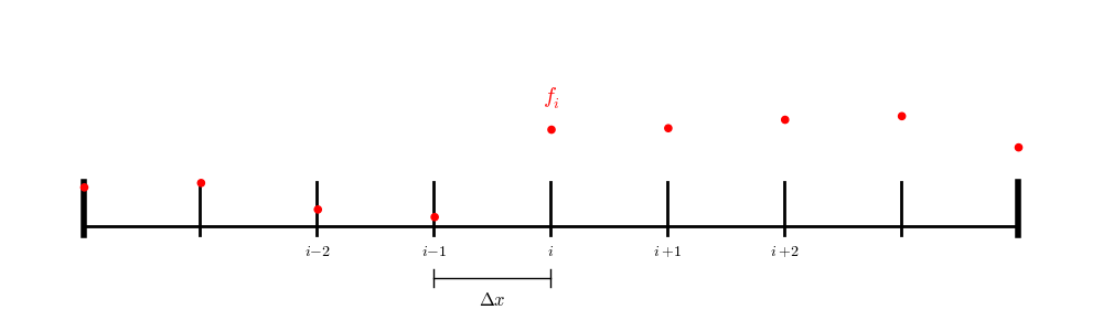
we have a point exactly on each boundary, so we only need to iterate over the interior points.

In contracts, for a finite-volume or cell-centered finite-difference grid:

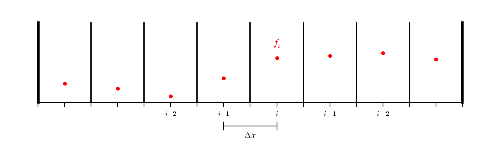
we don’t have data on the physical boundaries, so we will need to interpolate to the boundary.

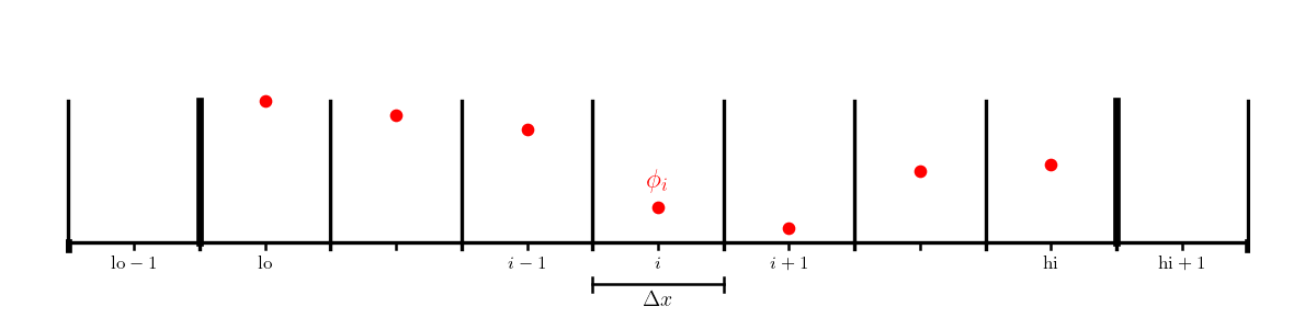
We’ll work with a cell-centered grid, with a single ghost cell (needed to set the boundary conditions). We’ll label the first interior zone as lo and the last interior zone as hi. Imagine that the domain runs from \([a, b]\).

Consider the following boundary conditions:

• Dirichlet: we need the value on the boundary itself to satisfy the boundary condition:

  \[\phi(a) = A\]

  A naive guess would be to set \(\phi_{\mathrm{lo}-1} = A\), but this is only first order accurate.

  Instead we recognize that we can average across the boundary to be second-onder on the boundary:

  \[A = \frac{\phi_\mathrm{lo} + \phi_\mathrm{lo-1}}{2}\]

  which gives the ghost cell value:

  \[\phi_{\mathrm{lo}-1} = 2 A - \phi_\mathrm{lo}\]

• Neumann: we need a gradient, centered at the boundary to match the given value:

  \[\phi^\prime(a) = C\]

  A second-order accurate discretization on the boundary is:

  \[C = \frac{\phi_\mathrm{lo} - \phi_\mathrm{lo-1}}{\Delta x}\]

  so we would initialize the ghost cell as:

  \[\phi_{\mathrm{lo}-1} = \phi_\mathrm{lo} -\Delta x C\]