
Homework 3 solutions#
We want to integrate the simple pendulum without the small angle approximation and compare different integration schemes. Our system is:
where \(\theta\) is the angular displacement from vertical and \(\omega\) is the angular velocity. The angular acceleration in this case is \(\alpha = -(g/L) \sin\theta\).
Note
Just like with the orbits, the angular acceleration, \(\alpha\), does not depend on (angular) velocity, \(\omega\). This means that we can use the symplectic integrators we looked at.
Our initial conditions are:
import numpy as np
import matplotlib.pyplot as plt
We’ll do everything in a single class, SimplePendulum, which will only store the initial conditions.
The actual integration history will be created and returned by the integration methods contained
in SimplePendulum, which allows us to create a single object and then run each of the 3 integration
methods from it for comparison.
class SimplePendulum:
    """ manage and integrate a simple pendulum """

    def __init__(self, theta0, g=9.81, L=9.81):
        """we'll take theta0 in degrees and assume that the angular
        velocity is initially 0"""

        # initial condition
        self.theta0 = np.radians(theta0)

        self.g = g
        self.L = L

    def energy(self, theta_vec, omega_vec):
        """ given a solution, return the energy (per unit mass) """
        return (0.5 * self.L**2 * omega_vec**2 -
                self.g * self.L * np.cos(theta_vec))

    def period(self):
        """ return an estimate of the period, up to the theta**2 term """
        return (2.0 * np.pi * np.sqrt(self.L / self.g) *
                (1.0 + self.theta0**2 / 16.0 +
                 11.0 * self.theta0**4 / 3072.0))

    def rhs(self, theta, omega):
        """ equations of motion for a pendulum
              dtheta/dt = omega
              domega/dt = - (g/L) sin theta """

        return np.array([omega, -(self.g / self.L) * np.sin(theta)])

    def integrate_ec(self, dt, tmax):
        """integrate the equations of motion using the Euler-Cromer method"""

        # initial conditions
        t = 0.0

        t_s = [t]
        theta_s = [self.theta0]
        omega_s = [0.0]

        while t < tmax:

            dt = min(dt, tmax-t)

            # initial state
            theta = theta_s[-1]
            omega = omega_s[-1]

            # get the RHS
            thetadot, omegadot = self.rhs(theta, omega)

            # advance
            omega_new = omega + dt * omegadot
            theta_new = theta + dt * omega_new

            t += dt

            # store
            t_s.append(t)
            theta_s.append(theta_new)
            omega_s.append(omega_new)

        return np.array(t_s), np.array(theta_s), np.array(omega_s)

    def integrate_vv(self, dt, tmax):
        """integrate the equations of motion using velocity Verlet method"""

        # initial conditions
        t = 0.0

        t_s = [t]
        theta_s = [self.theta0]
        omega_s = [0.0]

        while t < tmax:

            dt = min(dt, tmax-t)

            # initial state
            theta = theta_s[-1]
            omega = omega_s[-1]

            # get the RHS at time-level n
            thetadot, omegadot = self.rhs(theta, omega)

            omega_half = omega + 0.5 * dt * omegadot

            theta_new = theta + dt * omega_half

            # get the RHS with the updated theta -- omega doesn't matter
            # here, since we only need thetadot and omega doesn't affect
            # that.
            _, omegadot_new = self.rhs(theta_new, omega)
            omega_new = omega_half + 0.5 * dt * omegadot_new

            t += dt

            # store
            t_s.append(t)
            theta_s.append(theta_new)
            omega_s.append(omega_new)

        return np.array(t_s), np.array(theta_s), np.array(omega_s)

    def integrate_rk4(self, dt, tmax):
        """integrate the equations of motion using 4th order Runge Kutta"""

        # initial conditions
        t = 0.0

        t_s = [t]
        theta_s = [self.theta0]
        omega_s = [0.0]

        while t < tmax:

            dt = min(dt, tmax-t)

            # initial state
            theta = theta_s[-1]
            omega = omega_s[-1]

            # get the RHS at time-level n
            thetadot1, omegadot1 = self.rhs(theta, omega)

            theta_tmp = theta + 0.5 * dt * thetadot1
            omega_tmp = omega + 0.5 * dt * omegadot1

            thetadot2, omegadot2 = self.rhs(theta_tmp, omega_tmp)

            theta_tmp = theta + 0.5 * dt * thetadot2
            omega_tmp = omega + 0.5 * dt * omegadot2

            thetadot3, omegadot3 = self.rhs(theta_tmp, omega_tmp)

            theta_tmp = theta + dt * thetadot3
            omega_tmp = omega + dt * omegadot3

            thetadot4, omegadot4 = self.rhs(theta_tmp, omega_tmp)

            theta_new = theta + dt / 6.0 * (thetadot1 + 2.0 * thetadot2 +
                                            2.0 * thetadot3 + thetadot4)
            omega_new = omega + dt / 6.0 * (omegadot1 + 2.0 * omegadot2 +
                                            2.0 * omegadot3 + omegadot4)

            t += dt

            # store
            t_s.append(t)
            theta_s.append(theta_new)
            omega_s.append(omega_new)

        return np.array(t_s), np.array(theta_s), np.array(omega_s)
Let’s try it out
Case 1: \(\theta_0 = 10^\circ\)#
# initial angle in degrees -- the class converts to radians
theta0 = 10

p10 = SimplePendulum(theta0)
period = p10.period()
print(f"{period=}")
period=np.float64(6.295168481931661)
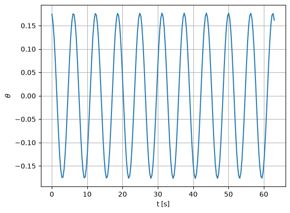
Euler-Cromer method
# fixed timestep
dt = period / 20
tmax = 10 * period
t_ec, theta_ec, omega_ec = p10.integrate_ec(dt, tmax)
fig, ax = plt.subplots()
ax.plot(t_ec, theta_ec, label="Euler-Cromer")

ax.set_xlabel("t [s]")
ax.set_ylabel(r"$\theta$")

ax.grid()
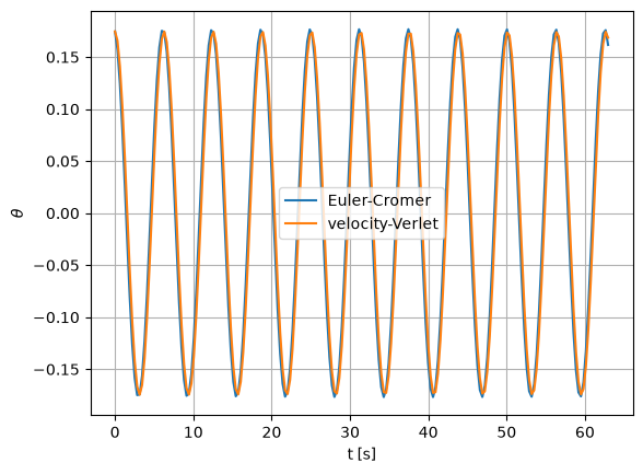
now velocity-Verlet
t_vv, theta_vv, omega_vv = p10.integrate_vv(dt, tmax)

ax.plot(t_vv, theta_vv, label="velocity-Verlet")
ax.legend()
fig
and finally 4th-order Runge-Kutta
t_rk4, theta_rk4, omega_rk4 = p10.integrate_rk4(dt, tmax)

ax.plot(t_rk4, theta_rk4, label="RK4")
ax.legend()
fig
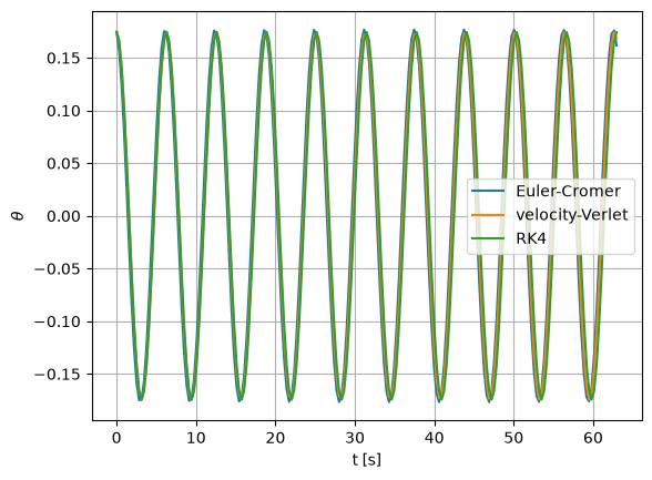
All the curves are quite close, but we see by the end there are some differences.
Let’s run for 100 periods and look at the last 10
tmax *= 10
t_ec2, theta_ec2, omega_ec2 = p10.integrate_ec(dt, tmax)
t_vv2, theta_vv2, omega_vv2 = p10.integrate_vv(dt, tmax)
t_rk42, theta_rk42, omega_rk42 = p10.integrate_rk4(dt, tmax)
fig, ax = plt.subplots()
ax.plot(t_ec2, theta_ec2, label="Euler-Cromer")
ax.plot(t_vv2, theta_vv2, label="velocity-Verlet")
ax.plot(t_rk42, theta_rk42, label="RK4")

ax.set_xlabel("t [s]")
ax.set_ylabel(r"$\theta$")
ax.set_xlim(90*period, 100*period)
ax.legend()
ax.grid()
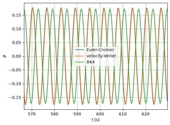
So we see that after a while, the two symplectic integrators stay in phase, but the RK4 integrator is completely out of phase.
Let’s look at energy for the original (10 periods) runs
E_ec = p10.energy(theta_ec, omega_ec)
E_vv = p10.energy(theta_vv, omega_vv)
E_rk4 = p10.energy(theta_rk4, omega_rk4)

fig = plt.figure()

ax1 = fig.add_subplot(211)
ax1.plot(t_ec, E_ec, label="Euler-Cromer")
ax1.grid()
ax1.legend()
ax1.set_ylabel("E/m")

ax2 = fig.add_subplot(212)
ax2.plot(t_vv, E_vv, label="velocity-Verlet")
ax2.plot(t_rk4, E_rk4, label="RK4")
ax2.grid()
ax2.legend()
ax2.set_xlabel("time")
ax2.set_ylabel("E/m")
Text(0, 0.5, 'E/m')
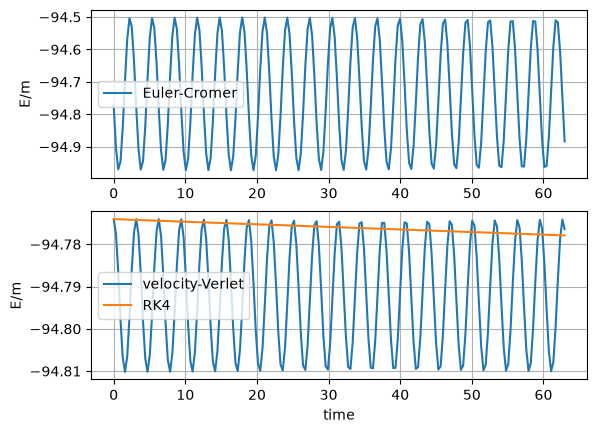
These are plotted on different scales since the Euler-Cromer method has much larger swings in the energy. But note that for both the Euler-Cromer and velocity-Verlet methods, the energy stays bounded and returns back to its original value each period.
For the 4th-order Runge-Kutta, there is a steady drift in the total energy.
Case 2: \(\theta_0 = 100^\circ\)#
theta0 = 100

p100 = SimplePendulum(theta0)
period = p100.period()
print(f"{period=}")
period=np.float64(7.688181618459404)
Notice that the period here is very different than the classic small-angle approximation period.
# fixed timestep
dt = period / 20
tmax = 10 * period
t_ec, theta_ec, omega_ec = p100.integrate_ec(dt, tmax)
t_vv, theta_vv, omega_vv = p100.integrate_vv(dt, tmax)
t_rk4, theta_rk4, omega_rk4 = p100.integrate_rk4(dt, tmax)
fig, ax = plt.subplots()

ax.plot(t_ec, theta_ec, label="Euler-Cromer")
ax.plot(t_vv, theta_vv, label="velocity-Verlet")
ax.plot(t_rk4, theta_rk4, label="RK4")

ax.legend()
ax.set_xlabel("t [s]")
ax.set_ylabel(r"$\theta$")

ax.grid()
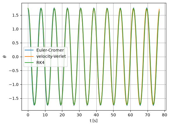
Again, the Euler-Cromer and velocity-Verlet methods track nicely
We’ll split the energy plot into 2 so we can better see the trends
E_ec = p100.energy(theta_ec, omega_ec)
E_vv = p100.energy(theta_vv, omega_vv)
E_rk4 = p100.energy(theta_rk4, omega_rk4)

fig = plt.figure()
ax1 = fig.add_subplot(211)

ax1.plot(t_ec, E_ec, label="Euler-Cromer")
ax1.legend()
ax1.grid()
ax1.set_ylabel("E/m")

ax2 = fig.add_subplot(212)
ax2.plot(t_vv, E_vv, label="velocity-Verlet")
ax2.plot(t_rk4, E_rk4, label="RK4")
ax2.legend()
ax2.grid()
ax2.set_xlabel("time")
ax2.set_ylabel("E/m")
Text(0, 0.5, 'E/m')
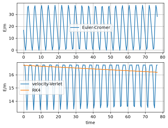
We see that, again, the two sympletic integrators seem to conserve energy over the period, but the 4th order Runge-Kutta has a steady drift just like we saw in the earlier case.
Convergence#
We’ll focus just on the larger amplitude. In addition to making a plot, we’ll also print out the difference between the minimum and maximum energy over the integration duration. This will be our metric for assessing convergence.
p = SimplePendulum(100)

fig, ax = plt.subplots()
for n in [20, 40, 80]:
    tau = p.period() / n
    t, theta, omega = p.integrate_ec(tau, 10*p.period())
    E = p.energy(theta, omega)
    ax.plot(t, p.energy(theta, omega), label=f"N = {n}")
    print(f"{n} : {E.max() - E.min()}")
ax.legend()
ax.grid()
ax.set_xlabel("time")
ax.set_ylabel("E/m")
20 : 37.873464677642545
40 : 18.69023944326237
80 : 9.314754417201456
Text(0, 0.5, 'E/m')
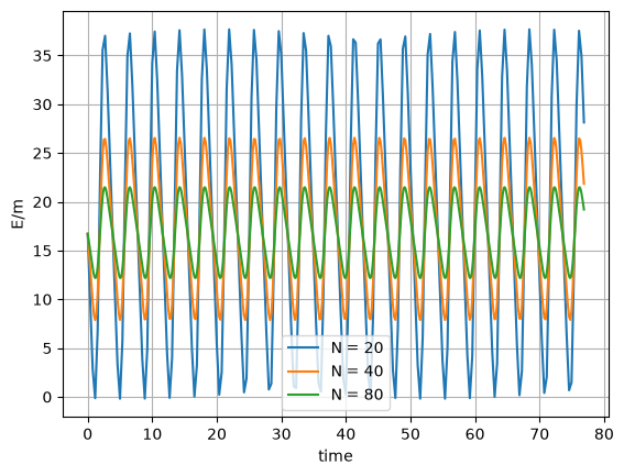
Notice that when we print out the amplitude of the energy, it decreases by a factor of 2 each time we double \(N\)—this is first-order convergence.
p = SimplePendulum(100)

fig, ax = plt.subplots()
for n in [20, 40, 80]:
    tau = p.period() / n
    t, theta, omega = p.integrate_vv(tau, 10*p.period())
    E = p.energy(theta, omega)
    ax.plot(t, E, label=f"N = {n}")
    print(f"{n} : {E.max() - E.min()}")
ax.legend()
ax.grid()
ax.set_xlabel("time")
ax.set_ylabel("E/m")
20 : 3.4088291065175973
40 : 0.8483208900033361
80 : 0.21185146597349913
Text(0, 0.5, 'E/m')
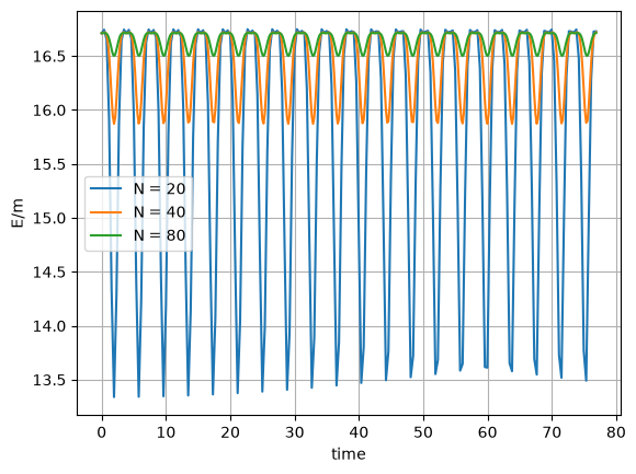
Now notice that when we print out the amplitude of the energy change over the integration, it decreases by a factor of 4 each time we double \(N\)—this is 2nd-order convergence.
p = SimplePendulum(100)

fig, ax = plt.subplots()
for n in [20, 40, 80]:
    tau = p.period() / n
    t, theta, omega = p.integrate_rk4(tau, 10*p.period())
    E = p.energy(theta, omega)
    ax.plot(t, E, label=f"N = {n}")
    print(f"{n} : {E.max() - E.min()}")
ax.legend()
ax.grid()
ax.set_xlabel("time")
ax.set_ylabel("E/m")
20 : 0.5346620582999186
40 : 0.017873506652158255
80 : 0.0005985955513878594
Text(0, 0.5, 'E/m')
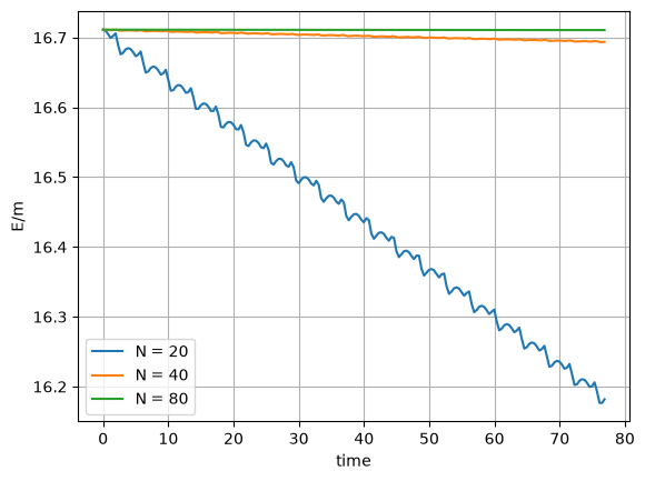
This now seems to be converging better than 4th order, even though the solution is clearly not as good as the other methods.