Lagrange Interpolation

Imagine that we have a dataset with \(N\) points, \(\{x_0, x_1, \ldots, x_{N-1}\}\) and associated function values \(\{f_0, f_1, \ldots, f_{N-1}\}\). We can write a general polynomial interpolation routine that passes through all \(N\) points using the Lagrange polynomial.

The basic idea is to create \(N\) basis functions of the form:

\[\ell_i(x) = \prod_{j=0, i\ne j}^{N-1} \frac{x - x_j}{x_i - x_j}\]

This has the property that:

\[\ell_i(x_j) = \delta_{ij}\]

We can then write our interpolant as:

\[f(x) = \sum_{i=0}^{N-1} \ell_i f_i\]

Quadratic example

Consider fitting a quadratic to three points:

\[(x_0, f_0), (x_1,f_1), (x_2, f_2)\]

Let’s imagine that they are evenly spaced, with a spacing \(\Delta x\).

The three basis functions are:

\[\begin{align*} \ell_0 &= \frac{x - x_1}{x_0 - x_1} \cdot \frac{x-x_2}{x_0 - x_2} = \frac{(x-x_1)(x-x_2)}{2 \Delta x^2} \\ \ell_1 &= \frac{x - x_0}{x_1 - x_0} \cdot \frac{x-x_2}{x_1 - x_2} = -\frac{(x-x_0)(x-x_2)}{\Delta x^2} \\ \ell_2 &= \frac{x - x_0}{x_2 - x_0} \cdot \frac{x-x_1}{x_2 - x_1} = \frac{(x-x_0)(x-x_1)}{2 \Delta x^2} \end{align*}\]

and the quadratic polynomial is:

\[ f(x) = \frac{(x-x_1)(x-x_2)}{2 \Delta x^2} f_0 - \frac{(x-x_0)(x-x_2)}{\Delta x^2} f_1 + \frac{(x-x_0)(x-x_1)}{2 \Delta x^2} f_2 \]

Let’s implement this

import numpy as np
import matplotlib.pyplot as plt

def f_lagrange(xeval, x, f):
    """ x, f are the 3 points, xeval is where we want to evaluate """
    dx = x[1] - x[0]

    return (xeval - x[1])*(xeval-x[2])*f[0]/(2.0*dx**2) - \
           (xeval - x[0])*(xeval-x[2])*f[1]/(dx**2) + \
           (xeval - x[0])*(xeval-x[1])*f[2]/(2.0*dx**2)

We’ll look at several different sets of points. For each, we’ll plot the interpolated parabola through the 3 points.

fig, ax = plt.subplots()

# grid points where our data is
x = np.array([0.0, 0.5, 1.0])

f1 = np.array([1.0, -1.0, 1.0/3.0])
f2 = np.array([0.5, 0.5, 0.1])
f3 = np.array([-0.3, 1.3, 1.0])

xfine = np.linspace(0.0, 1.0, 200)

for farray in (f1, f2, f3):
    ax.scatter(x, farray, marker="x", s=25)
    ax.plot(xfine, f_lagrange(xfine, x, farray))

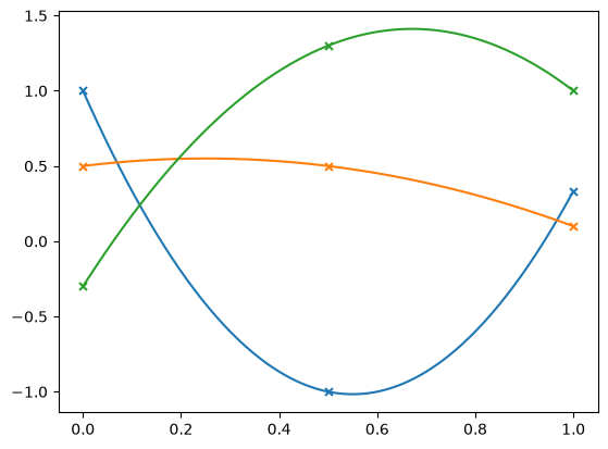
Notice that the interpolated values exceed the range of \(\{f_1, f_2, f_3\}\). For some applications we may not to introduce new extrema.

Lagrange interpolation is not very computationally efficient, since you need to recompute the basis functions for each point. There are more efficient ways to compute this, like barycentric form that are algebraically equivalent.

Runge’s phenomena

Lagrange interpolation also suffers from Runge’s phenomenon if used with equally spaced points. This gives rise to larges osciallations at the end of the interpolating interval if we use very high-order polynomial.

Let’s write a general Lagrange interpolation class and test it out on some different functions.

class LagrangePoly:
    """ a general class for creating a Lagrange polynomial 
    representation of a function """

    def __init__(self, xmin, xmax, N, func, chebyshev=False):
        self.N = N
        self.xmin = xmin
        self.xmax = xmax
        self.func = func

        if chebyshev:
            k = np.arange(N) + 1
            self.xp = 0.5 * (xmin + xmax) + 0.5 * (xmax - xmin) * np.cos((2 * k -1) * np.pi / (2 * N))
        else:
            self.xp = np.linspace(self.xmin, self.xmax, self.N)
        self.fp = func(self.xp)

    def evalf(self, x):
        """ given a point x and a function func, fit a Lagrange
        polynomial through the control points and return the
        interpolated value at x """

        f = 0.0

        # sum over points
        for m in range(len(self.xp)):

            # create the Lagrange basis polynomial for point m
            l = 1

            for n in range(len(self.xp)):
                if n == m:
                    continue

                l *= (x - self.xp[n])/(self.xp[m] - self.xp[n])

            f += self.fp[m]*l

        return f

Let’s test it out on a \(\tanh\) profile

def func(x):
    return 0.5 * (1.0 + np.tanh((x - 1.0) / 0.1))

N = 11
xmin = 0.0
xmax = 2.0

l = LagrangePoly(xmin, xmax, N, func)

Let’s compute the interpolated value at a lot of points and also compute the error with respect to the exact function value.

# xx are the finely grided data that we will interpolate at to get
# the interpolated function values ff
xx = np.linspace(xmin, xmax, 200)
ff = np.zeros_like(xx)

for n, v in enumerate(xx):
    ff[n] = l.evalf(v)

# exact function values at the interpolated points
fexact = func(xx)

def plot_result(xx, ff, fexact):

    # compute the error
    e = fexact - ff

    fig = plt.figure()
    ax = fig.add_subplot(211)

    ax.scatter(l.xp, l.fp, marker="x", s=30)
    ax.plot(xx, ff)

    ax.plot(xx, fexact, color="0.5")

    ax = fig.add_subplot(212)

    ax.plot(xx, e)
    ax.set_xlabel("x")
    ax.set_ylabel("error")
    fig.tight_layout()

plot_result(xx, ff, fexact)

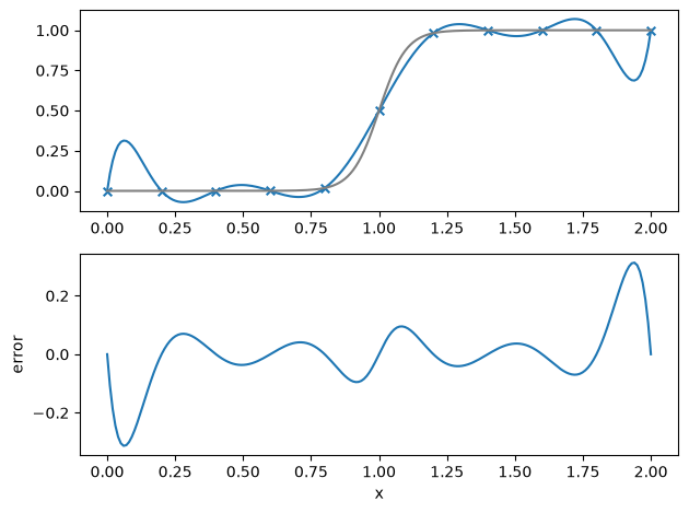
What happens as we increase the number of data samples, \(N\)?

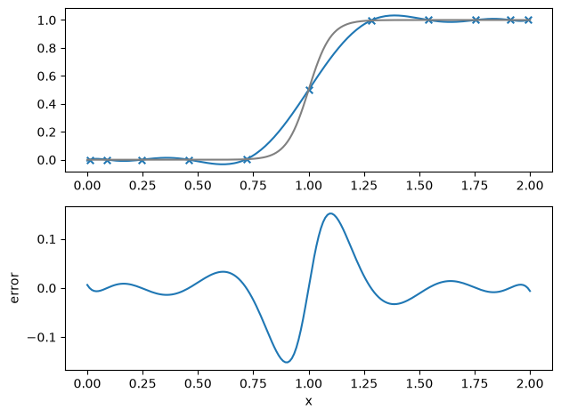
Chebyshev nodes

If we are free to pick the points where we sample the function, we can do a lot better, and minimize the Runge’s phenomena. Sampling \(f(x)\) at the Chebyshev nodes:

\[x_k = \frac{1}{2}(a +b) + \frac{1}{2} (b-a) \cos \left (\frac{2k - 1}{2n}\pi \right )\, , \quad k = 1, \ldots n\]

where \([a, b]\) is the domain, works well.

Let’s try this out

l = LagrangePoly(xmin, xmax, N, func, chebyshev=True)

for n, v in enumerate(xx):
    ff[n] = l.evalf(v)

# exact function values at the interpolated points
fexact = func(xx)

plot_result(xx, ff, fexact)