Least Squares Regression

Imagine a dataset where we have a set of points, \((x_i, y_i)\) with associated errors in \(y\), \(\sigma_i\), and we want to fit a line or curve to them.

Our data looks like:

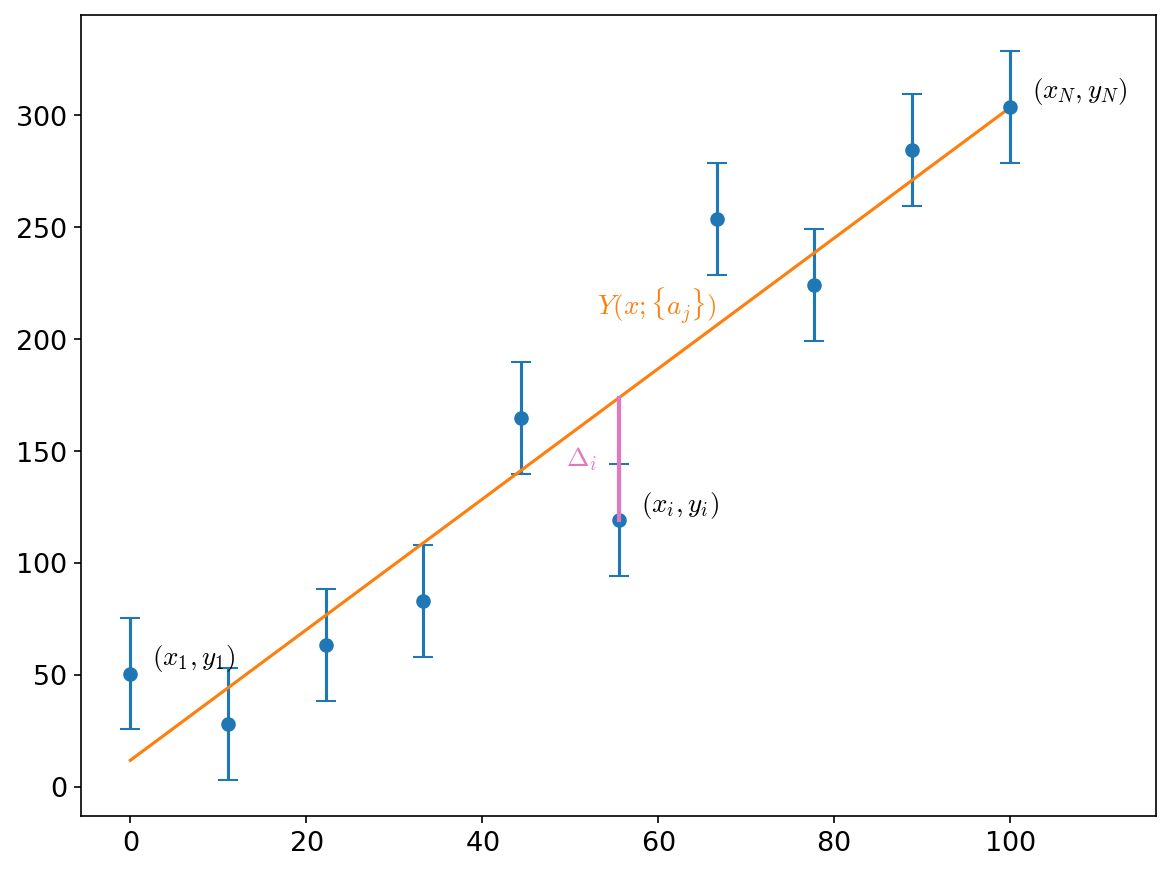
Fig. 3 Set of points and associated errors

We want to create a model, \(Y(x; {a_j})\) that best fits these points. Here the values \({a_j}\) are free parameters that we will tune to get a good fit.

For each point, we will measure the vertical distance to the model:

\[\Delta_i = Y(x_i; {a_j}) - y_i\]

and we want to minimize the distance. We do this by defining

\[\chi^2({a_j}) \equiv \sum_i \left(\frac{\Delta_i}{\sigma_i}\right )^2\]

Here, each point’s distance, \(\Delta_i\) is weighted by its error, \(\sigma_i\) — this ensures that points that we are least certain of has less influence in the fit. Minimizing \(\chi^2\) with respect to the fit parameters, \({a_j}\) is called least squares minimization.

The minimization procedure involves setting the derivatives of \(\chi^2\) with respect to each of the \({a_j}\) to zero and solving the resulting system.

For linear least squares, all of the \({a_j}\) enter into \(Y(x; {a_j})\) linearly, e.g., as:

\[Y(x; {a_j}) = a_1 + a_2 x + a_3 x^2\]

And the minimization process results in a linear system that can be solved using the techniques we learned when we discussed linear algebra.

Note

Even though this polynomial \(Y\) here is nonlinear in \(x\), it is linear in \(a_j\), which means that this is still a case of linear least squares.

The special case of fitting a line:

\[Y(x; {a_j}) = a_1 + a_2 x\]

is called linear regression.

For nonlinear least squares, the parameters can enter in a nonlinear fashion, and the solution methodology is considerably more complex.

Take care…

Fitting can be misleading, and you should always think about what the data is saying and how it relates to the function you are fitting to:

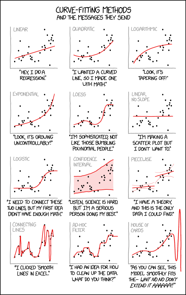
Fig. 4 Image: XKCD