
Application: Interpolating Weak Reaction Rate Tables#
Supernovae shine because of the radioactive decay of \({}^{56}\mathrm{Ni}\), which is one of the end-points of fusion reactions of light elements. At high densities, once this \({}^{56}\mathrm{Ni}\) is made, the electron-capture reaction:
is important in determining how much \({}^{56}\mathrm{Ni}\) remains compared to other stable iron-group nuclei. A similar transformation can happen via \(\beta^+\) decay:
Note
We call these reactions weak nuclear reactions, because they involve changing a neutron to a proton, and thus the weak nuclear force.
These reaction rates are temperature and density dependent (in terms of electron density, \(\rho Y_e\), where \(Y_e\) is the electron fraction) and evaluations of them are usually provided as tables requiring reaction networks to interpolate.
Here we’ll learn how to work with a tabulated reaction rate.
Accessing the data#
Here’s a table for the above rates: 56ni-56co_electroncapture.dat from Langanke & Martínez-Pinedo 2001. This has been cleaned up a little
from the tables provided there, combining both the e-capture and \(\beta^+\)-decay into a single rate.
import numpy as np
!head 56ni-56co_electroncapture.dat
#56ni -> 56co, e- capture
#Q=-1.624 MeV
#
#Log(rhoY)    Log(temp)     mu              dQ    Vs     Log(e-cap-rate)        Log(nu-energy-loss)  Log(gamma-energy)
#Log(g/cm^3)  Log(K)        erg             erg   erg    Log(1/s)               Log(erg/s)           Log(erg/s)
1.000000      7.000000      -4.806530e-09  0.00  0.00   -8.684000              -1.486129e+01         -100.00
1.000000      8.000000      -9.292624e-08  0.00  0.00   -9.164000              -1.533229e+01         -100.00
1.000000      8.301030      -2.146917e-07  0.00  0.00   -9.291000              -1.544729e+01         -100.00
1.000000      8.602060      -4.902661e-07  0.00  0.00   -9.387000              -1.551729e+01         -100.00
1.000000      8.845098      -8.058948e-07  0.00  0.00   -8.777000              -1.485829e+01         -100.00
We see that the data is in columns with most quantities stored as logs. We’re interest in the first column, \(\log(\rho Y_e)\), the second column, \(\log(T)\), and the sixth column, \(\log(\lambda)\) (the reaction rate).
Note
The \(\log()\) are base-10 logarithms.
Tip
We’ll use np.genfromtxt() to read this, which can interpret a comment line as labels for the data, giving us an
easy way to index the columns.
data = np.genfromtxt("56ni-56co_electroncapture.dat", skip_header=3, names=True)
From the table, we can learn that there are 13 temperatures and 11 densities in the tabulation.
ntemp = 13
nrho = 11
We can extract the unique densities (\(\log(\rho Y_e)\)) from the LogrhoY column, by taking every ntemp value:
logrho = data["LogrhoY"][::ntemp]
logrho
array([ 1., 2., 3., 4., 5., 6., 7., 8., 9., 10., 11.])
and the unique temperatures (\(\log(T)\)) from the Logtemp column:
logT = data["Logtemp"][0:ntemp]
logT
array([ 7.      ,  8.      ,  8.30103 ,  8.60206 ,  8.845098,  9.      ,
        9.176091,  9.30103 ,  9.477121,  9.69897 , 10.      , 10.477121,
       11.      ])
Note
The temperatures are not evenly spaced. We need to make sure that we take that into account when we do the interpolation.
Finally, we’ll access the rate, \(\lambda\), from the Logecaprate column, and reshape it into a two-dimensional table:
lograte = data["Logecaprate"].reshape(nrho, ntemp)
Here are a few of the values:
lograte[0:4, 0:4]
array([[-8.684, -9.164, -9.291, -9.387],
       [-7.705, -8.165, -8.291, -8.387],
       [-6.834, -7.171, -7.293, -7.388],
       [-6.118, -6.22 , -6.31 , -6.392]])
In this form, density varies in the first dimension (across rows) and temperature varies in the second dimension (across columns).
Bilinear interpolation#
We’ll do bilinear interpolation, using taking the 4 points in the table that surround the \((\rho Y_e, T)\) at which we wish to evaluate the rate and fit it with a function:
here we take \((i, j)\) as the reference point for the interpolant.
We need to find the 4 unknowns, \(\{a, b, c, d\}\), using the information from the table.
Visually, this appears as:
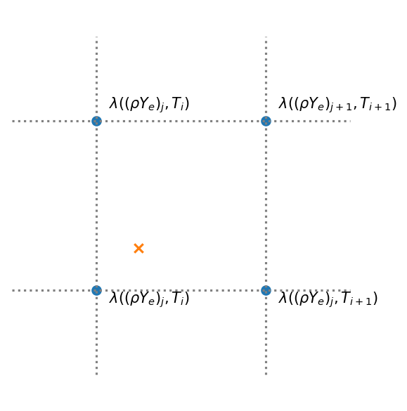
where the \(\times\) is where we want to know the rate.
We can do this algebraically, by evaluating our interpolant at our 4 points:
Then we see:
Here’s an implementation of this interpolation:
def interp(logrhoY_v, logT_v, lograte_t, logrhoY0, logT0):
    """interpolate lograte_t to find the rate at a point (logrhoY0, logT0).
    Here logrhoY_v and logT_v are the points where the rate is tabulated"""

    i = np.argwhere(logrhoY_v > logrhoY0)[0][0] - 1
    j = np.argwhere(logT_v > logT0)[0][0] - 1

    dlogrhoY = logrhoY_v[i+1] - logrhoY_v[i]
    dlogT = logT_v[j+1] - logT_v[j]

    a = (lograte_t[i+1, j+1] - lograte_t[i+1, j] - lograte_t[i, j+1] + lograte_t[i, j]) / (dlogrhoY * dlogT)
    b = (lograte_t[i+1, j] - lograte_t[i, j]) / dlogrhoY
    c = (lograte_t[i, j+1] - lograte_t[i, j]) / dlogT
    d = lograte_t[i, j]

    return (a * (logrhoY0 - logrhoY_v[i]) * (logT0 - logT_v[j]) +
            b * (logrhoY0 - logrhoY_v[i]) +
            c * (logT0 - logT_v[j]) +
            d)
Caution
We do nothing to check that the density and temperature are contained within the table and don’t fall out of bounds of the table limits.
Now we can try it.
logrhoY0 = 3.5
logT0 = 9.4
loglambda = interp(logrho, logT, lograte, logrhoY0, logT0)
loglambda
np.float64(-4.7833819981855985)
print(f"at T = {10**logT0:12.6g} and (rho Y_e) = {10**logrhoY0:12.6g}, the rate is {10**loglambda:12.6g}")
at T = 2.51189e+09 and (rho Y_e) = 3162.28, the rate is 1.64671e-05
Using SciPy#
We can do the same bilinear interpolation using SciPy.
from scipy import interpolate
lrate = interpolate.interpn((logrho, logT), lograte, (3.5, 9.4))
10**lrate
array([1.64671333e-05])
We see that we get the same value (to at least 7 significant digits!)
SciPy can also do bicubic interpolation–this would require 16 points instead of the 4 points our method used.
lrate = interpolate.interpn((logrho, logT), lograte, (3.5, 9.4), method="cubic")
10**lrate
array([1.58899208e-05])
We see that this differs from the bilinear value in the second significant digit.