Homework 6 solutions

We want to solve Burgers’ equation using two different first-order difference approximations. We’ll write a single class that has both updates. First we’ll do the grid—we can essentially reuse the grid from our linear advection solver, but change the boundary conditions to be outflow.

import numpy as np
import matplotlib.pyplot as plt

class FDGrid:
    """a finite-difference grid"""

    def __init__(self, nx, ng=1, xmin=0.0, xmax=1.0):
        """create a grid with nx points, ng ghost points (on each end)
        that runs from [xmin, xmax]"""

        self.xmin = xmin
        self.xmax = xmax
        self.ng = ng
        self.nx = nx

        # python is zero-based.  Make easy integers to know where the
        # real data lives
        self.ilo = ng
        self.ihi = ng+nx-1

        # physical coords
        self.dx = (xmax - xmin)/(nx-1)
        self.x = xmin + (np.arange(nx+2*ng)-ng)*self.dx

        # storage for the solution
        self.u = np.zeros((nx+2*ng), dtype=np.float64)
        self.uinit = np.zeros((nx+2*ng), dtype=np.float64)
        
    def scratch_array(self):
        """ return a scratch array dimensioned for our grid """
        return np.zeros((self.nx+2*self.ng), dtype=np.float64)

    def fill_BCs(self):
        """ fill the a single ghostcell with outflow """
        self.u[self.ilo-1] = self.u[self.ilo]
        self.u[self.ihi+1] = self.u[self.ihi]

Now the Burgers’ solver. Again we’ll base this on the upwind advection case, but with a few changes:

• The timestep computation needs to look at the maximum velocity and be considered each step

• The update itself is now different

• There is no sense of a period, since we are doing outflow BCs, so we pass in the maximum time

• We don’t pass in the advective velocity, since for Burgers’ equation, velocity is the quantity on the grid itself

def burgers_solve(nx, C, tmax, init_cond=None, method="conservative"):
    """solve Burgers' equation with either a conservative or non-conservative
    difference method"""
    
    g = FDGrid(nx)
    
    # time info
    t = 0.0

    # initialize the data
    init_cond(g)

    g.fill_BCs()
    g.uinit[:] = g.u[:]
    
    # evolution loop
    unew = g.scratch_array()

    while t < tmax:

        dt = C * g.dx / np.abs(g.u).max()
        
        if t + dt > tmax:
            dt = tmax - t

        # fill the boundary conditions
        g.fill_BCs()

        # loop over zones and do the update
        if method == "conservative":
            unew[g.ilo:g.ihi+1] = g.u[g.ilo:g.ihi+1] - \
                0.5 * dt * (g.u[g.ilo:g.ihi+1]**2 - g.u[g.ilo-1:g.ihi]**2) / g.dx
            
        elif method == "non-conservative":
            unew[g.ilo:g.ihi+1] = g.u[g.ilo:g.ihi+1] - \
                dt * g.u[g.ilo:g.ihi+1] * (g.u[g.ilo:g.ihi+1] - g.u[g.ilo-1:g.ihi]) / g.dx
            
        else:
            raise ValueError(f"solution method {method} not defined")

        # store the updated solution
        g.u[:] = unew[:]
        
        t += dt
    
    # fill the ghost cells for the returned object
    g.fill_BCs()
    return g

Our initial conditions are the same as the shock initial conditions we saw in class

def shock(g):
    g.u[:] = 2.0
    g.u[g.x > 0.5] = 1.0

Conservative solution

nx = 64
tmax = 0.2
C = 0.8

g = burgers_solve(nx, C, tmax, init_cond=shock)

fig, ax = plt.subplots()
ax.plot(g.x, g.u)
ax.plot(g.x, g.uinit, ls=":", label="initial conditions")
ax.legend()

<matplotlib.legend.Legend at 0x7fc9fc3f0070>

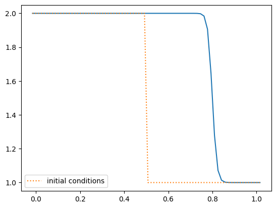
Let’s write a simple function to compute the shock speed by simply finding the first zone where the velocity drops below 1.5 and differencing that location at the different times

def shock_speed(g, tmax):
    x0 = g.x[g.uinit <= 1.5][0]
    x1 = g.x[g.u <= 1.5][0]
    return (x1 - x0) / tmax

Now let’s see how the shock speed behaves with resolution

for nx in [64, 128, 256, 512]:
    g = burgers_solve(nx, C, tmax, init_cond=shock)
    speed = shock_speed(g, tmax)
    print(f"nx: {nx:4}, shock speed = {speed:7.3f}")

nx:   64, shock speed =   1.508
nx:  128, shock speed =   1.496
nx:  256, shock speed =   1.490
nx:  512, shock speed =   1.497

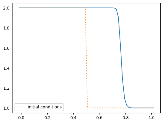
Non-conservative update

nx = 64
tmax = 0.2
C = 0.8

g = burgers_solve(nx, C, tmax, init_cond=shock, method="non-conservative")

fig, ax = plt.subplots()
ax.plot(g.x, g.u)
ax.plot(g.x, g.uinit, ls=":", label="initial conditions")
ax.legend()

<matplotlib.legend.Legend at 0x7fc9fc3aa020>

for nx in [64, 128, 256, 512]:
    g = burgers_solve(nx, C, tmax, init_cond=shock, method="non-conservative")
    speed = shock_speed(g, tmax)
    print(f"nx: {nx:4}, shock speed = {speed:7.3f}")

nx:   64, shock speed =   1.349
nx:  128, shock speed =   1.339
nx:  256, shock speed =   1.373
nx:  512, shock speed =   1.370

Summary

We know the correct shock speed for this—our initial conditions are just a Riemann problem and we derived the shock speed for that via the Rankine-Hugoniot jump conditions:

\[S = \frac{1}{2} (u_l + u_r)\]

so for our problem the shock speed is \(S = 1.5\).

We see that the conservatively differenced method gets the correct shock speed but the non-conservative method does not. The reason for this is that the shock represents a discontinuity where the derivative \(\partial u / \partial x\) is not defined. The conservative formulation matches the finite-volume method, where we use the flux difference to compute the update. This casts the equation in integral rather than differential form, where the discontinuity is not a problem.