Root Finding#
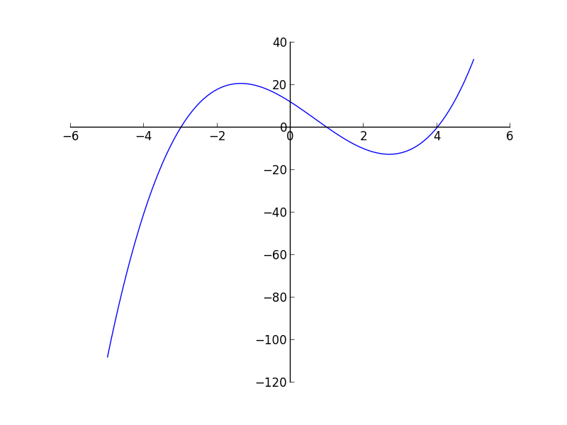
Given a function \(f(x)\), the root-finding problem is to find all of the \(x\) such that \(f(x) = 0\).
Root finding algorithms often need a range that bracket the root, \(x_0\), i.e. \(x_0 \in [x_l, x_r]\).
Notice that (for most functions) near \(f(x) = 0\), \(f(x)\) changes sign, so often we will check that \(f(x_l) \cdot f(x_r) < 0\).
There are a large number of root finding algorithms.
Bisection#
Bisection works by iteratively cutting the range where the root is located in half. The basic idea is as follows:
Iterate until error is small:
Compute \(f_l = f(x_l)\) and \(f_r = f(x_r)\)
Define \(x_m = (x_l + x_r) / 2\) and \(f_m = f(x_m)\)
If \(f_l \cdot f_m < 0\) then the \(x_0 \in [x_l, x_m]\), so define \(x_r = x_m\); otherwise set \(x_l = x_m\)
Define the error as \(|x_r - x_l|\)
Here’s an animation of bisection finding a root:
Bisection is slow to converge—it only reduces the error by a factor of 2 each iteration.
Note
Bisection will fail to find the root for \(f(x) = x^2\).
Newton’s method#
For Newton’s method, we start by Taylor expanding the function about some initial guess for the root, \(x_0\):
if \(x_0\) is close to the actual root, then \(\delta x\) is a correction that will bring it closer to the actual root, and the higher order terms in this expansion will be small, so we can neglect them. This tells us that the correction is:
Then we can correct our guess:
and iterate on this procedure until \(|\delta x|\) is small.
Here’s an animation showing the method converging:
There are a few things to note here:
The initial guess needs to be good—if it is not, then the higher order terms, which start with \(\delta x^2\) are not small, and we should not have neglected them.
We need a good estimate of the derivative. Ideally this means that we supply a function that computes the derivative analytically.
Newton’s method can fail in a variety of ways, including entering a cycle.
Note
If we don’t have an analytic form of the derivative, then we can compute it via finite-differences. This can give rise to the secant method.
Implementation#
We want to write a function that takes as input the function we want to zero, so we’ll
use std::function to define the function as an argument.
Here’s the header that implements both bisection and Newton’s method:
#ifndef ROOTS_H
#define ROOTS_H

#include <iostream>
#include <functional>
#include <cmath>

namespace Roots {
    const double ATOL = 1.e-10;   // absolute tolerance
    const double RTOL = 1.e-10;   // relative tolerance
    const int MAX_ITER = 100;
}

///
/// Apply bisection to find a root of f(x) in the range [xleft, xright]
/// Return value is 0 if root found, non-zero if there was an error
///
int bisection(double xleft, double xright,
              std::function<double(double)> f,
              double& root) {

    int ierr{0};

    double fleft = f(xleft);
    double fright = f(xright);

    if (fleft * fright > 0) {
        std::cout << "no root in interval [xleft, right]" << std::endl;
        ierr = 1;
        return ierr;
    } else if (fleft == 0 || fright == 0) {
        std::cout << "root is one of bounds" << std::endl;
        ierr = 1;
        return ierr;
    }

    double xmid = 0.5 * (xleft + xright);

    int iter{0};

    while (iter < Roots::MAX_ITER) {
        double fmid = f(xmid);

        if (fleft * fmid > 0.0) {
            // root is in [fmid, fright]
            xleft = xmid;
        } else {
            // root is in [fleft, fmid]
            xright = xmid;
        }

        double err = std::abs(xright - xleft);
        xmid = 0.5 * (xleft + xright);

        if (err < Roots::RTOL * std::abs(xmid) + Roots::ATOL) {
            ierr = 0;
            break;
        }

        iter++;
    }

    root = xmid;

    return ierr;
}

///
/// Apply Newtons's method to find a root of f(x) starting with the initial
/// guess x0.  In addition to f(x) we need to supply the derivative, dfdx(x).
/// Return value is 0 if root found, non-zero if there was an error
///
int newton(double x0,
           std::function<double(double)> f,
           std::function<double(double)> dfdx,
           double& root) {

    int ierr{1};

    double f0 = f(x0);
    double dfdx0 = dfdx(x0);

    root = x0;

    int iter{0};

    while (iter < Roots::MAX_ITER ) {

        double dx = -f0/dfdx0;

        if (std::abs(dx) < Roots::RTOL * std::abs(x0) + Roots::ATOL) {
            ierr = 0;
            root = x0;
            break;
        }

        x0 += dx;

        f0 = f(x0);
        dfdx0 = dfdx(x0);

        iter++;
    }

    return ierr;
}
#endif
A few features:
We use a
namespaceto hold the parameters that affect the behavior of the root finding algorithms. This ensures that if we#include "roots.H"in a file, these names don’t conflict with any that might be locally defined.We use both a relative and absolute tolerance for assessing the error. Convergence is met when:
\[\epsilon < \mathrm{RTOL} |x_0| + \mathrm{ATOL}\]This ensures that if the current estimate of the root, \(x_0\), is close to zero then \(\mathrm{ATOL}\) is used but if the root \(x_0\) is large, then \(\mathrm{RTOL}\) use used for the error.
We have a maximum number of iterations,
Roots::MAX_ITER, after which we exit with an error. This ensures we don’t get stuck in an infinite loop if something goes wrong.
Here’s a test driver for it:
#include <iostream>

#include "roots.H"

int main() {

    int ierr{0};
    double root{0.0};

    // bisection on f(x) = x^3 + x^2 - 1

    std::cout << "trying bisection on f(x) = x^3 + x^2 - 1" << std::endl;

    ierr = bisection(-5.0, 5.0,
                     [] (double x) {return x*x*x + x*x - 1.0;}, root);

    if (ierr == 0) {
        std::cout << root << std::endl;
    } else {
        std::cout << "root not found" << std::endl;
    }
    std::cout << std::endl;


    // bisection on f(x) = x^2

    std::cout << "trying bisection on f(x) = x^2" << std::endl;

    ierr = bisection(-5.0, 5.0,
                     [] (double x) {return x*x;}, root);

    if (ierr == 0) {
        std::cout << root << std::endl;
    } else {
        std::cout << "root not found" << std::endl;
    }
    std::cout << std::endl;


    // Newton's method on f(x) = x^2

    std::cout << "trying Newton's method on f(x) = x^2" << std::endl;

    ierr = newton(-1.0,
                  [] (double x) {return x*x;}, [] (double x) {return 2*x;}, root);

    if (ierr == 0) {
        std::cout << root << std::endl;
    } else {
        std::cout << "root not found" << std::endl;
    }
    std::cout << std::endl;

}
Note
What happens if we use \(x_0 = 0\) as the initial guess for \(f(x) = x^2\) with Newton’s method?
try it…
Write a version of Newton’s method that uses a finite-difference approximation to the derivative.