Introduction to Parallel Programming#
Modern computers have multiple CPU cores. So far, we’ve only been doing work on a single core, but a lot of computational physics numerical work can be spread across multiple CPUs.
Moore’s law#
Moore observed that over time, the number of transistors that can be packed into a chip doubled roughly every two years.

Fig. 16 (Max Roser, Hannah Ritchie, Our World In Data, Wikipedia)#
These extra transistors can go into additional logic (vector units, etc.), more cache, or increasing the number of cores. Presently, individual cores are not getting much faster from one year to the next, but the number of cores packed into a chip is increasing considerably (especially if you consider GPUs too).
In fact, increases in single-threaded CPU performance have greatly slowed:
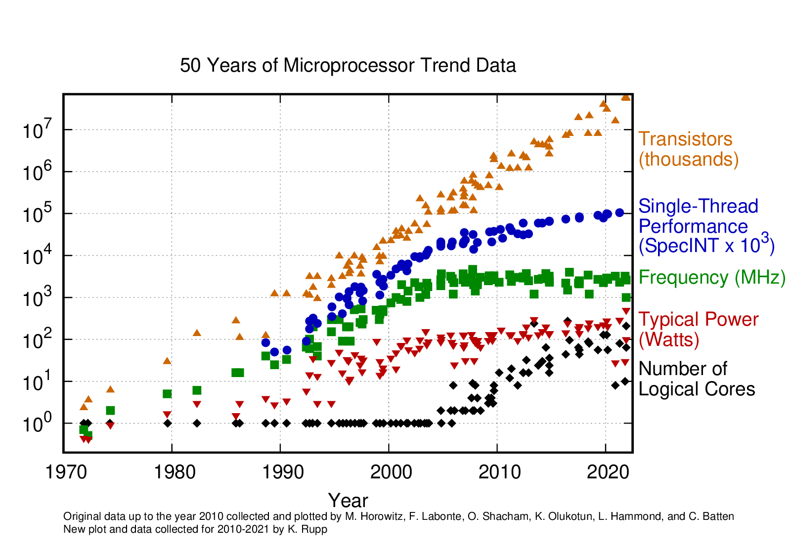
Fig. 17 Figure from karlrupp/microprocessor-trend-data#
This means that to effectively take advantage of new processors, we need to put these additional cores to work.
Looking at the Top 500 list also shows the trends in how the fastest computers are changing.
Memory architecture#
A lot of the considerations in parallel program involve how we access the memory where the data is stored. There are generally two approaches:
shared memory: all computing cores have direct access to the memory (perhaps not all with the same speed though)
OpenMP is a popular approach here.
distributed memory: the memory is separated in ways that only certain cores can access certain pools of memory. This could be, for example, because the computer is a cluster comprised of multiple computers (nodes) connected via a high-speed network.
MPI is a popular approach here.
Often we will do a little of each—shared memory parallelism inside a compute node and distributed memory parallelism across nodes.
There is another type of parallelism—using accelerators, like GPUs, that dominates high performance computing now. Here we can use OpenMP, OpenACC, or a vendor-specific library like CUDA or HIP to do the offloading.
Tip
Sometimes when moving computation to work in parallel we need to change the algorithm we are using. We’ll see an example of this shortly.
Amdahl’s law#
In a typical application, you’ll have sections of code that adapt easily to parallelism and stuff that does not, and remains serial.
E.g., initialization might be serial but computation is parallel
Amdahl’s law gives the theoretical speed up of a code when running on \(N\) processors, given the fraction of the code that is parallel, P:
For example:
\(P = 0.5\) (half of our code can be executed in parallel):
N
S
1
1.0
2
1.333
4
1.6
8
1.778
16
1.882
32
1.940
\(P = 0.9\) (90% of our code can be executed in parallel):
N
S
1
1.0
2
1.818
4
3.077
8
4.706
16
6.400
32
7.805
Does this mean that we have no hope of using machines with 100,000’s of cores? No:
New algorithms have been designed to exploit massive parallelism
Larger computers mean bigger problems are possible—as you increase the problem size, the fraction of the code that is serial likely decreases.
Types of parallelism#
Flynn’s taxonomy categorizes the different types of parallelism.
4 classifications: single/multiple data; single/multiple instruction:
Single instruction, single data (SISD)
Think typical application on your computer—no parallelism
Single instruction, multiple data (SIMD)
The same instruction set is done to multiple pieces of data all at once
Old days: vector computers; today: GPUs
Multiple instructions, single data (MISD)
Not very interesting…
Multiple instructions, multiple data (MIMD)
What we typically think of as parallel computing.
The machines on the top 500 list fall into this category
MIMD#
We can do MIMD different ways:
Single program, multiple data:
This is what we normally do.
MPI allows this.
Differs from SIMD in that general CPUs can be used.
Doesn’t require direct sync of all tasks
Trivially parallel#
Sometimes no communication is needed between processes—this is trivially parallel
Examples:
Ray tracing or Monte Carlo:
Each realization can do its work independently
At the end, maybe we need to do some simple processing of all of the results
Analyzing a large collection of data files
We have a pipeline that works on a single file—we can run multiple pipelines each on a separate file.
Each file is processed on a single core.
Making your code parallel#
There is no magic compiler flag that makes your code run in parallel. So your approach really depends on what you are doing and where you intend to run.
Runtime dominated by one task#
Imagine that the majority of your runtime is dominated by a single task (like linear algebra). You can get a good speed up just by switching to a library that does the linear algebra in parallel. This requires minimal code changes.
Shared memory#
Imagine that we want to run on a single computer that has one CPU (one socket on the motherboard) with multiple cores. Each of these cores will have direct access to the same pool of memory:
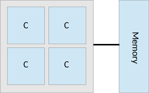
Fig. 18 A single 4-core chip and its pool of memory#
In this situation, the parallelism is straightforward:
Allocate a single big array for your problem
Spawn threads: separate instance of a sequence of instructions operating
Multiple threads operate simultaneously
Each core/thread operates on a smaller portion of the same array, writing to the same memory
Some intermediate variables may need to be duplicated on each thread—thread-private data
OpenMP is the standard here.
Note
Some machines are more complex—multiple chips each with their own pool of local memory. The chips can talk to one another through a slower connection, so accessing memory “off chip” could slow you down.
Best performance requires knowing your machine’s architecture.
Distributed memory#
With distributed memory, we run on a collection of computers, connected by a high-speed network.
Each task cannot directly see the memory for the other tasks
Need to explicitly send messages from one machine to another over the network exchanging the needed data
MPI is the standard here.