Example: Planetary Orbit

Let’s consider an example of integrating the orbit of Earth around the Sun (we’ll consider the mass of the Earth to be tiny compared to the Sun so we can neglect the Sun’s motion around the center of mass).

Kepler’s third law tells us:

\[4\pi^2 a^3 = G M_\star P^2\]

where \(a\) is the semi-major axis and \(P\) is the period of the orbit. If we work in units of solar masses, astronomical units, and years, then this becomes:

\[a^3 = P^2\]

which implies that \(G M_\star = 4 \pi^2\).

The evolution of the planet is given by

\[\dot{\bf r} = {\bf v}\]

\[\dot{\bf v} = - \frac{G M_\star {\bf r}}{r^3}\]

where \({\bf r} = (x, y)\) and \({\bf v} = (v_x, v_y)\).

Euler’s Method

The simplest method to advance the solution begins with a first-order accurate difference approximation to the derivative:

\[\frac{{\bf r}^{n+1} - {\bf r}^n}{\tau} = {\bf v}^n + \mathcal{O}(\tau)\]

\[\frac{{\bf v}^{n+1} - {\bf v}^n}{\tau} = {\bf a}({\bf r}^n,{\bf v}^n) + \mathcal{O}(\tau)\]

or

\[{\bf r}^{n+1} = {\bf r}^n + \tau {\bf v}^n + \mathcal{O}(\tau^2)\]

\[{\bf v}^{n+1} = {\bf v}^n + \tau {\bf a}({\bf r}^n,{\bf v}^n) + \mathcal{O}(\tau^2)\]

This shows that each time we take a step, we make an error (called truncation error) of \(\mathcal{O}(\tau^2)\). Over the course of the orbit we will take \(N = T / \tau\) steps, so the global error will be \(\mathcal{O}(\tau)\).

This method is first-order accurate in time.

Graphically, Euler’s method looks like:

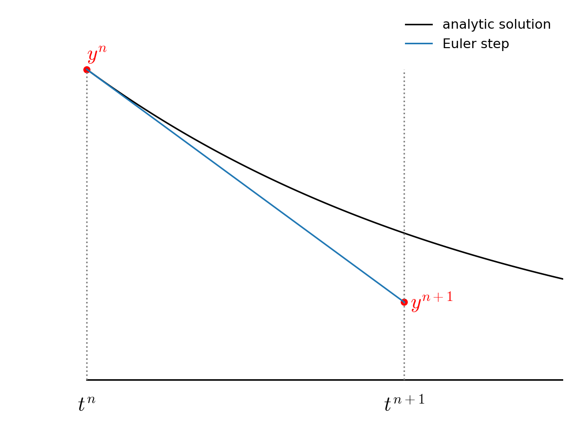
Fig. 7 Euler’s method: we evaluate the slope at the start of the timestep and then follow this through to the new time.

Implementation

We’ll store the state of the solution at a single instance in time in a struct:

struct OrbitState {
    double t;
    double x;
    double y;
    double vx;
    double vy;
};

and we’ll save the solution at each step in a vector:

std::vector<OrbitState> orbit_history{};

This corresponds to the “array-of-structs” storage scheme we discussed earlier.

To make our code flexible, we’ll write the following functions:

• A righthand side function, with the forward declaration:

  OrbitState rhs(const OrbitState& state);
  

  we can evaluate this as needed by passing in an OrbitState and returning the derivative of that state with respect to time.

• A function to write out the history:

  void write_history(const std::vector<OrbitState>& history);
  

  We can adapt this as desired to write to the screen or a file.

• An integration function:

  std::vector<OrbitState> integrate(const double a, const double tmax, const double dt);
  

  This manages the time-stepping, implementing Euler’s method and storing the solution in our history vector each step. At the end of integration it will return the history.

try it…

Implement the solver by filling in the details of the functions described above.

solution

Listing 33 orbit_example.cpp

#include <iostream>
#include <iomanip>
#include <vector>
#include <cmath>

struct OrbitState {
    double t;
    double x;
    double y;
    double vx;
    double vy;
};

OrbitState rhs(const OrbitState& state);
void write_history(const std::vector<OrbitState>& history);
std::vector<OrbitState> integrate(const double a, const double tmax, const double dt_in);

const double GM = 4.0 * M_PI * M_PI;   // G * Mass in AU, year, solar mass units

OrbitState rhs(const OrbitState& state) {

    OrbitState dodt{};

    // dx/dt = vx; dy/dt = vy

    dodt.x = state.vx;
    dodt.y = state.vy;

    // d(vx)/dt = - GMx/r**3; d(vy)/dt = - GMy/r**3

    double r = std::sqrt(state.x * state.x + state.y * state.y);

    dodt.vx = - GM * state.x / std::pow(r, 3);
    dodt.vy = - GM * state.y / std::pow(r, 3);

    return dodt;

}

void write_history(const std::vector<OrbitState>& history) {

    for (auto o : history) {
        std::cout << std::setw(12) << o.t
                  << std::setw(12) << o.x
                  << std::setw(12) << o.y
                  << std::setw(12) << o.vx
                  << std::setw(12) << o.vy << std::endl;

    }

}

std::vector<OrbitState> integrate(const double a, const double tmax, const double dt_in) {

    // how the history of the orbit

    std::vector<OrbitState> orbit_history{};

    // set initial conditions
    OrbitState state{};

    // assume circular orbit on the x-axis, counter-clockwise orbit

    state.t = 0.0;
    state.x = a;
    state.y = 0.0;
    state.vx = 0.0;
    state.vy = std::sqrt(GM / a);

    orbit_history.push_back(state);

    double dt = dt_in;

    // integration loop
    while (state.t < tmax) {

        if (state.t + dt > tmax) {
            dt = tmax - state.t;
        }

        // get the derivatives
        auto state_derivs = rhs(state);

        // update the state
        state.t += dt;
        state.x += state_derivs.x * dt;
        state.y += state_derivs.y * dt;
        state.vx += state_derivs.vx * dt;
        state.vy += state_derivs.vy * dt;

        orbit_history.push_back(state);
    }

    return orbit_history;

}

int main() {

    double tmax = 1.0;
    double dt = 0.001;
    double a = 1.0;      // 1 AU

    auto orbit_history = integrate(a, tmax, dt);
    write_history(orbit_history);

}

Tip

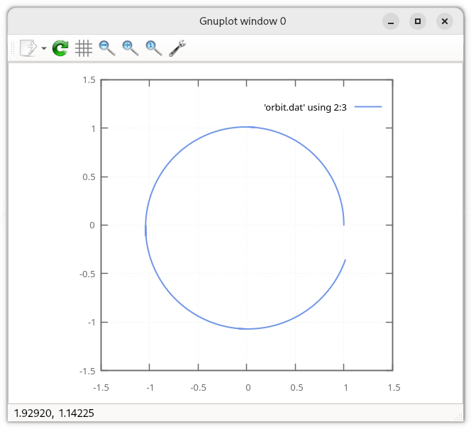
We can plot the solution using gnuplot.

First, when you run, redirect the output to a file:

./orbit_example > orbit.dat

Now run gnuplot:

gnuplot

A simple plot in gnuplot is made using the plot command, specifying the file with the data, the columns to use for x and y axes, and any styling (like w l for with-lines):

plot 'orbit.dat' using 2:3 w l
set size square
replot

This will make something like:

You can save the plot as:

set term png
set output "orbit.png"
replot

For more info, see: http://www.gnuplot.info/