Adaptive Runge-Kutta#
Previously we looked at the simple Euler and 2nd-order Runge-Kutta methods for integration. Now we will look at 4th order Runge-Kutta. We will also:
Write our integrator as a class that works with any ODE system of the form:
\[\frac{d{\bf y}}{dt} = {\bf f}(t, {\bf y})\]Adapt the timestep taken internally to achieve a user-desired error in the solution.
4th order RK#
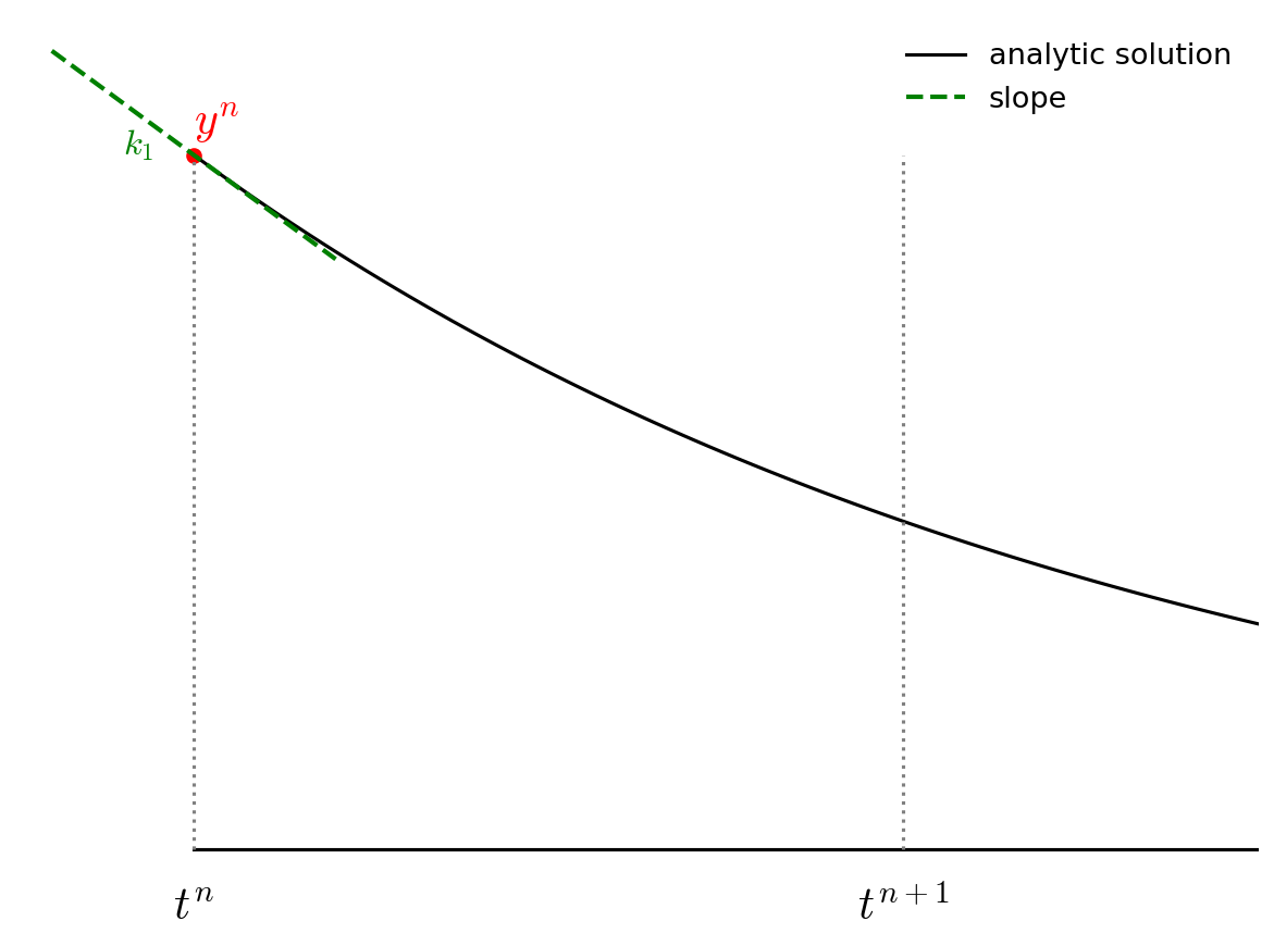
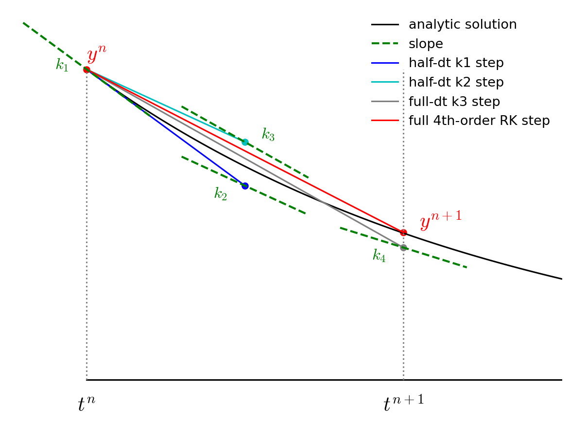
Fourth-order Runge-Kutta consists of 4 stages and a final update, illustrated below:
The advance begins by estimating the derivatives (righthand side or slope) at time \(t^n\). We’ll call this \({\bf k}_1\).
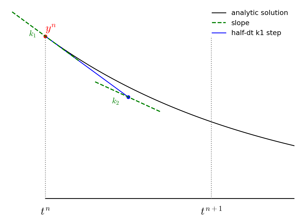
We then follow the slope \({\bf k}_1\) to the midpoint in time, \(t^{n+1/2}\) and evaluate the slope there. We call the new slope \({\bf k}_2\).
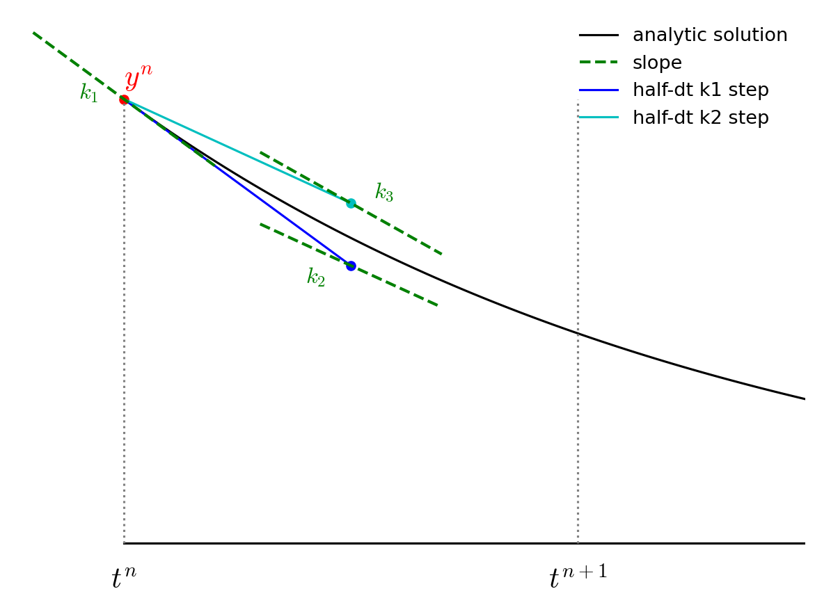
We then go back to the start, but this time follow the new slope, \({\bf k}_2\) to the midpoint in time, \(t^{n+1/2}\). We again evaluate the slope here, and call it \({\bf k}_3\).
Finally, we go back to the start and follow \({\bf k}_3\) for the full timestep, to \(t^{n+1}\) and evaluate the slope there, calling it \({\bf k}_4\).
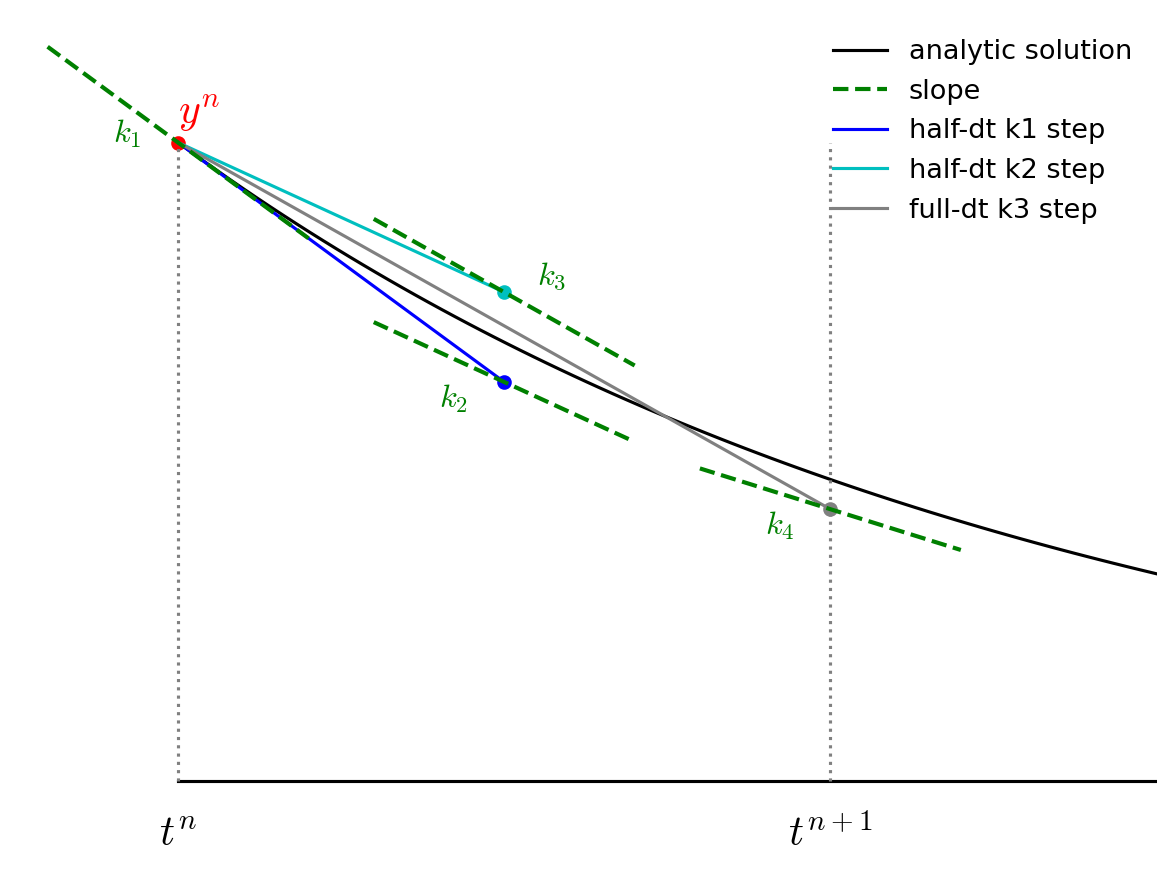
We then get the updated solution using a linear combination of the 4 slopes:
Note the similarity of RK4 to Simpson’s rule for integration.
Adaptive timesteps#
So far we’ve been integrating with a fixed timestep. This gives us no real control over the error. What we would like to do is take a small timestep when the solution is changing fast, and a larger timestep when the solution changes more slowly.
To do this, we need to be able to assess the error in our solution as we integrate. There are lots of different ways to do this in the literature:
Take two half steps and compare to one full step
Compare higher and lower order methods (sometimes the lower order method is embedded in the higher-order method, for instance this is the RK45 method used by SciPy).
We’ll do the first method here, as it is the simplest. Consider integrating a function \(y(t)\) through some timestep \(\tau\):
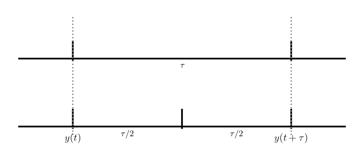
Fig. 14 Adaptive timestep comparing \(\tau/2\) steps to a single \(\tau\) step.#
The top evolution takes a single step of size \(\tau\) while the bottom takes two steps each of \(\tau/2\). These two integrations both end at \(y(t+\tau)\), but we expect the one that took 2 half steps to be more accurate (since the truncation error is smaller).
Now, we know that RK4 is locally 5th order accurate, so that means that for our single step, the error will be:
And imagine that we wanted to achieve an error of \(\epsilon_\mathrm{want}\)—there is a timestep \(\tau_\mathrm{est}\) that would get this:
If we take the ratio of these, then any proportionality cancels, and we have
If we were not accurate enough, this would predict a finer timestep that would give us our desired accuracy. And if we were too accurate, then this would tell us how much we could increase the timestep while maintaining our desired accuracy.
Let’s consider doing this with RK4. Our approach will be:
Integrate from \(y(t)\) to \(y(t+\tau)\) using a single timestep, \(\tau\).
Call the solution \(y^\mathrm{single}\)
Integrate from \(y(t)\) to \(y(t+\tau)\) using two steps of size \(\tau/2\).
Call the solution \(y^\mathrm{double}\)
Compute an estimate of the relative error in the solution as:
\[\epsilon_\mathrm{rel} = \left | \frac{y^\mathrm{double} - y^\mathrm{single}} {y^\mathrm{double}} \right |\]Compute the timestep that would give us our desired accuracy, \(\epsilon_\mathrm{want}\):
\[\tau_\mathrm{est} = \tau \left (\frac{\epsilon_\mathrm{want}}{\epsilon_\mathrm{rel}} \right)^{1/5}\]If \(\epsilon_\mathrm{rel} < \epsilon_\mathrm{want}\) then our timestep was good, and store the solution at time \(t + \tau\) as \(y^\mathrm{double}\). Increase the timestep according to \(\tau_\mathrm{est}\) for the next step.
If \(\epsilon_\mathrm{rel} > \epsilon_\mathrm{want}\) then throw away our solution and go back to \(y(t)\) and retry the integration with the new, smaller \(\tau_\mathrm{est}\).
In practice, we usually limit the amount that the timestep can change from one attempt to the next by a factor of \(\sim 4\) or so.
Note
For a different method, the timestep estimate will likely be different, since it depends on the scaling of the local truncation error with the timestep, \(\tau\).
Implementation#
Here’s the code:
ode_integrator.H
#ifndef ODE_INTEGRATOR_H
#define ODE_INTEGRATOR_H

#include <array>
#include <cassert>
#include <cmath>
#include <functional>
#include <iostream>
#include <iomanip>
#include <limits>
#include <ranges>
#include <vector>

// A 4th-order Runge-Kutta integrator to solve:
//
//   dy/dt = f
//   y(t=0) = y0
//
// where y is a vector of length N.
// This is templated on the size of the system, N.
//
// The signature of the righthand side function, f, is:
//
// std::vector<double> f(double t, const std::array<double>& y)
//

namespace adaptive_rk4 {
    constexpr double S1{0.9};
    constexpr double S2{4.0};
}

using rhs_func =
    std::function<std::vector<double>(double,
                                      const std::vector<double>&)>;

using rhs_param_func =
    std::function<std::vector<double>(double,
                                      const std::vector<double>&,
                                      std::vector<double>&)>;

struct solution {
    double t;
    std::vector<double> y{};

    // constructor that takes an vector of values

    solution(double t_in, std::vector<double>& y_in)
        : t(t_in), y(y_in) {}

};

std::ostream& operator<<(std::ostream& os, const solution& s) {
    os << std::setprecision(4);
    os << std::setw(10) << s.t << " ";
    for (auto e : s.y) {
        os << std::setw(10) << e << " ";
    }
    return os;
}

class ODE {

public:

    int neqs{-1};

    int n_rhs{0};
    int n_reset{0};
    double dt_min{std::numeric_limits<double>::max()};
    double dt_max{std::numeric_limits<double>::lowest()};

private:

    double t{0.0};

    std::vector<double> y_init;
    std::vector<double> params;
    rhs_func rhs;
    rhs_param_func rhs_param;

    std::vector<solution> history{};

    // do an update of the form y_new = y + dt * dydt

    std::vector<double> update_step(const std::vector<double>& y0, double dt,
                                    std::vector<double>& dydt) {

        std::vector<double> y_new{y0};
        for (auto n = 0ul; n < y_new.size(); ++n) {
            y_new[n] += dt * dydt[n];
        }

        return y_new;
    }

    // do a single step of RK4 given initial y0 and timestep dt

    std::vector<double> rk4_step(const std::vector<double>& y0, double t0, double dt) {

        // get the k1 acceleration
        auto k1 = params.empty() ? rhs(t0, y0) : rhs_param(t0, y0, params);
        n_rhs++;

        assert(static_cast<int>(k1.size()) == neqs);

        // get the k2 acceleration
        auto y_tmp = update_step(y0, 0.5*dt, k1);
        auto k2 = params.empty() ? rhs(t0 + 0.5*dt, y_tmp) : rhs_param(t0 + 0.5*dt, y_tmp, params);
        n_rhs++;

        // get the k3 acceleration
        y_tmp = update_step(y0, 0.5*dt, k2);
        auto k3 = params.empty() ? rhs(t0 + 0.5*dt, y_tmp) : rhs_param(t0 + 0.5*dt, y_tmp, params);
        n_rhs++;

        // get the k4 acceleration
        y_tmp = update_step(y0, dt, k3);
        auto k4 = params.empty() ? rhs(t0 + dt, y_tmp) : rhs_param(t0 + dt, y_tmp, params);
        n_rhs++;

        // compute the final update
        for (auto n = 0ul; n < y0.size(); ++n) {
            y_tmp[n] = y0[n] + (dt / 6.0) * (k1[n] + 2.0 * k2[n] + 2.0 * k3[n] + k4[n]);
        }

        return y_tmp;
    }


public:

    // constructor that takes an vector with initial conditions

    ODE(rhs_func rhs_in, std::vector<double> _y0)
        : neqs(_y0.size()), y_init(_y0), rhs(rhs_in)
    {
        history.emplace_back(t, y_init);
    }

    // constructor that takes an vector with initial conditions
    // and another with params that are passed to the RHS function

    ODE(rhs_param_func rhs_in, std::vector<double> _y0, std::vector<double> _p)
        : neqs(_y0.size()), y_init(_y0), params(_p), rhs_param(rhs_in)
    {
        history.emplace_back(t, y_init);
    }

    // integrate the system to tmax.  Here, dt_in is the initial
    // timestep.  The timestep will be adjusted internally to get a
    // relative tolerace or rtol.

    std::vector<solution>& integrate(double dt_in, double tmax, double rtol=1.e-6) {

        // start with the suggested timestep
        double dt_new{dt_in};
        double dt{dt_in};

        while (t < tmax) {

            const auto & sol_old = history.back();

            // adaptive timestepping loop -- keep trying to take a
            // step until we achieve our desired error
            double rel_error{std::numeric_limits<double>::max()};
            int n_try{};

            std::vector<double> y_new{};

            while (rel_error > rtol) {

                dt = dt_new;
                if (t + dt > tmax) {
                    dt = tmax - t;
                }

                // take 2 half steps

                auto y_tmp = rk4_step(sol_old.y, t, 0.5*dt);
                y_new = rk4_step(y_tmp, t + 0.5*dt, 0.5*dt);

                // now take a single step to cover dt
                auto y_single = rk4_step(sol_old.y, t, dt);

                // y_new should be more accurate, so we'll keep that if
                // the error is low

                rel_error = 0.0;
                for (auto n = 0ul; n < y_new.size(); ++n) {
                    rel_error = std::max(rel_error,
                                         std::abs((y_new[n] - y_single[n]) / y_new[n]));
                }

                // adaptive timestep algorithm
                double dt_est = adaptive_rk4::S1 * dt * std::pow(std::abs(rtol / rel_error), 0.2);
                dt_new = std::clamp(dt_est, dt / adaptive_rk4::S2, adaptive_rk4::S2 * dt);

                n_try++;
            }

            if (n_try > 1) {
                // there were resets
                n_reset += (n_try - 1);
            }

            dt_min = std::min(dt_min, dt);
            dt_max = std::max(dt_max, dt);

            t += dt;
            history.emplace_back(t, y_new);

        }
        return history;
    }

};

#endif
Note
With C++23 we can write things a little cleaner using std::views::zip(),
for example, replacing:
rel_error = 0.0;
for (auto n = 0ul; n < y_new.size(); ++n) {
     rel_error = std::max(rel_error,
                          std::abs((y_new[n] - y_single[n]) / y_new[n]));
}
with:
rel_error = 0.0;
for (const auto [yd, ys] : std::views::zip(y_new, y_single)) {
     rel_error = std::max(rel_error, std::abs((yd - ys) / yd));
}
Some notes:
We use
std::vectorinternally to store the data for the system of ODEs. We could have usedstd::array, but that would have required us to template theODEclass on the number of equations.At each point in time, the state of the system is stored in a
structcalledsolution. There is a simple constructor that can fill the data.We have an overload for the stream operation,
<<, that works with asolutionobject.Our righthand side function can have one of 2 signatures:
A simple function of the form \(f(t, y)\):
std::vector<double> f(double t, const std::vector<double>& y)
A version that allows for a vector of parameters, \(f(t, y, p)\):
std::vector<double> f(double t, const std::vector<double>& y,
                      std::vector<double>& params)
The second case allows us to pass a vector of parameters that the system may depend on that are not the integration variables. This is a common feature in ODE integrators.
We use emplace_back instead of
push_back()to add asolutionto our history vector. This eliminates the need to create a temporarysolutionobject to push to the vector (likely through a move), e.g., as:history.push_back(solution(t, y));
instead
emplace_backsimply passes the arguments we give it to the constructor and operates directly on the vector.The
ODEclass manages the solution. There are 2 constructors, one for each type of righthand side function. Each takes the set of initial conditions.
The basic usage is:
std::vector<double> y0(0.0, 1.0, 2.0);
o = ODE(f, y0);
auto history = o.integrate(dt, tmax);
The integrator will take the number of equations in the system from
the number of initial conditions, and it will expect that the
righthand side function, f returns a vector of this length (this
is asserted).
We can also use an initialization list like:
o = ODE(f, {0.0, 1.0, 2.0});
Finally, the integrate member function can optionally take the relative
tolerance with which to find the solution.
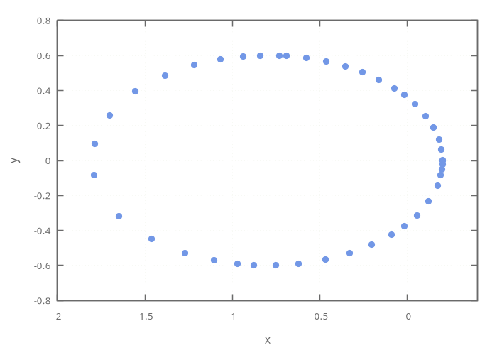
Example: elliptical orbits#
Here’s a driver for integrating orbits. We pick a high eccentricity which means that the planet’s speed will vary a lot over the orbit.
The initial conditions put the planet on the +x axis, at perihelion, with a counterclockwise orbit. They are:
#include <cmath>
#include <vector>
#include <iostream>

#include "ode_integrator.H"

enum orbit_comps {
    ix,
    iy,
    iu,
    iv};

constexpr double GM{4.0 * M_PI * M_PI};   // G * Mass in AU, year, solar mass unit

std::vector<double> orbit([[maybe_unused]] double t,
                          const std::vector<double>& y) {

    // order is x, y, u, v
    double dxdt = y[iu];
    double dydt = y[iv];

    // du/dt = - GMx/r**3; dv/dt = - GMy/r**3

    double r = std::sqrt(y[ix] * y[ix] + y[iy] * y[iy]);

    double dudt = - GM * y[ix] / std::pow(r, 3);
    double dvdt = - GM * y[iy] / std::pow(r, 3);

    return {dxdt, dydt, dudt, dvdt};

}

int main() {

    double a{1.0};
    double e{0.8};

    // planet is at perihelion initially

    double r_p = a * (1.0 - e);
    double v_p = std::sqrt(GM / a * (1.0 + e) / (1.0 - e));

    ODE o(orbit, {r_p, 0.0, 0.0, v_p});

    double tol{1.e-8};
    auto trajectory = o.integrate(0.025, 1.0, tol);

    std::cout << "# number of RHS evaluations = " << o.n_rhs << std::endl;
    std::cout << "# number of rejected steps = " << o.n_reset << std::endl;
    std::cout << "# dt range = [" << o.dt_min << ", " << o.dt_max << "]" << std::endl;

    for (const auto& s : trajectory) {
        std::cout << s << std::endl;
    }
}
Note
Notice that in our RHS function, we don’t explicitly create the std::vector
that we will return, but instead our return looks like:
return {dxdt, dydt, dudt, dvdt};
This is an example of using a braced initialization list for the return.
Tip
When run, the output will show the range of timesteps taken.
Here’s a plot of the output, showing the points computed during the solution. Notice that at perihelion they are much more closely spaced than at aphelion.
try it…
How does our solution compare (in terms of accuracy and number of steps) if we force the code to use a uniform timestep?
Example: Lorenz system#
Here’s a driver for integrating the Lorenz system. This system appears as:
and is a simple model for convection. Here, \(x\) is a measure of the rate of convection, \(y\) is related to the horizontal temperature variation, and \(z\) is related to the vertical temperature structure. There are 3 parameters: \(\sigma\) is the Prandtl number, \(\rho\) is the Rayleigh number, and \(\beta\) is related to the system size.
Lorenz chose \(\sigma = 10\), \(\beta = 8/3\), and \(\rho = 28\).
#include <vector>
#include <iostream>

#include "ode_integrator.H"

enum lorenz_comps {
    ix,
    iy,
    iz};

enum param_comps {
    isigma,
    irho,
    ibeta};

std::vector<double> rhs([[maybe_unused]] double t,
                        const std::vector<double>& y,
                        std::vector<double>& params) {

    double dxdt = params[isigma] * (y[iy] - y[ix]);
    double dydt = params[irho] * y[ix] - y[iy] - y[ix] * y[iz];
    double dzdt = y[ix] * y[iy] - params[ibeta] * y[iz];

    return {dxdt, dydt, dzdt};

}

int main() {

    // these are the parameters that Lorenz used

    constexpr double sigma{10.0};
    constexpr double rho{28.0};
    constexpr double beta{8.0/3.0};

    ODE o(rhs, {-10.0, -10.0, -10.0},
          {sigma, rho, beta});

    double tol{1.e-4};
    auto trajectory = o.integrate(0.025, 50.0, tol);

    std::cout << "# number of RHS evaluations = " << o.n_rhs << std::endl;
    std::cout << "# number of rejected steps = " << o.n_reset << std::endl;
    std::cout << "# dt range = [" << o.dt_min << ", " << o.dt_max << "]" << std::endl;

    for (const auto& s : trajectory) {
        std::cout << s << std::endl;
    }
}
The Lorenz system is interesting because it is chaotic—small changes to the initial conditions will lead to very large differences in the solution.
try it…
Try changing the initial conditions by \(1\) part in \(10^6\) and compare plots of \(x\) vs. \(t\).
Example: using a lambda-function#
For a simple system, we can use a lambda-function. Here we solve:
with \(y(0) = 1\).
#include <vector>
#include <iostream>

#include "ode_integrator.H"

// solve dy/dt = -y with y(0) = 1

int main() {

    auto f = [] (double t, const std::vector<double>& y) -> std::vector<double>
             {return {-y[0]};};

    ODE o(f, {1.0});

    double tol{1.e-8};
    auto trajectory = o.integrate(0.025, 1.0, tol);

    std::cout << "# number of RHS evaluations = " << o.n_rhs << std::endl;
    std::cout << "# number of rejected steps = " << o.n_reset << std::endl;
    std::cout << "# dt range = [" << o.dt_min << ", " << o.dt_max << "]" << std::endl;

    for (const auto& s : trajectory) {
        std::cout << s << std::endl;
    }
}