Poisson Equation and Relaxation#
We want to solve the Poisson equation:
We’ll do it in 1-d, writing our equation as:
on a domain \([a, b]\).
Note
This is a second-order PDE, so we need 2 boundary conditions.
We’ll use Dirichlet boundary conditions:
Discretization#
We will represent \(\phi\) and \(f\) on a 1-d uniform grid, with \(N\) points ranging from \(0, \ldots, N-1\):
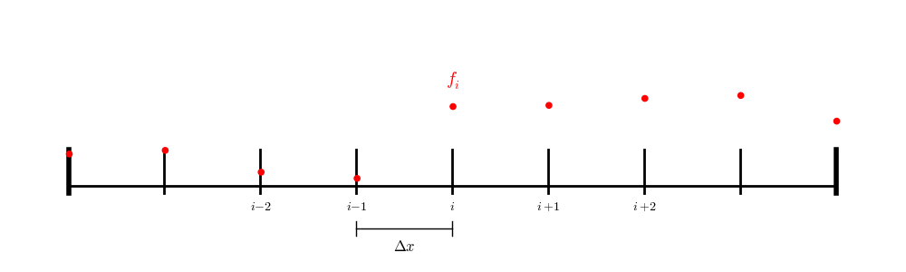
Fig. 15 Our 1-d finite difference grid#
Here we represent the discrete value of \(\phi\) with a subscript:
and similarly for \(f_i\).
Notice that with this grid we have a point on each boundary. We will set these points to the boundary conditions:
We now discretize the Poisson equation. Let’s start with the Taylor expansions for \(\phi_{i+1}\) and \(\phi_{i-1}\):
adding \(\phi_{i+1}\) and \(\phi_{i-1}\), we get:
which we can solve for:
This shows that our approximation to the second derivative is second-order accurate. We can then write the discrete Poisson equation as:
Since the boundary values are fixed, for a grid of \(N\) points, we need to update the points \(1, \ldots, N-2\) using this expression.
Note
Neumann boundary conditions are more complicated. If we want \(\phi^\prime(a) = 0\), then we use a second-order approximation to the derivative and a ghost point just outside the domain:
we also know from the Poisson equation:
Together these can be used to eliminate \(\phi_{-1}\) and give us an expression to use for \(\phi_0\):
Relaxation#
We can solve for the update for a single zone:
Our solution procedure is to iteratively apply this, updating the values \(\phi_i\) as we go along. This process is called relaxation or smoothing and the approach we will use, where we use the new information immediately as it becomes available is called Gauss-Seidel relaxation.
Stopping#
We need a measure to determine when we should stop relaxing the solution. We define the residual, \(r\), as:
This is a measure of how we’ll we satisfy the discrete equation.
We will keep iterating until the norm of the residual is small compared to the norm of the source:
Once that is satisfied, then we have solved the problem as well as we can do with the number of points we are using in the discretization.
This requires us to define a vector norm. We’ll use the L2 norm:
Note
The residual is telling us how well we solve the discrete form of the Poisson equation. It does not tell us if the discretization we chose to solve is good enough for our problem. For that, we would need to do convergence testing and/or comparisons to problems with known solutions.
Implementation#
Here’s a class that implements smoothing:
poisson.H
#ifndef POISSON_H
#define POISSON_H

#include <vector>
#include <cassert>
#include <cmath>
#include <limits>
#include <fstream>
#include <iomanip>
#include <functional>

///
/// Solve the 1-d Poisson problem on a node-centered finite-difference
/// grid with Dirichlet BCs using Gauss-Seidel smoothing
///
class Poisson {

private:

    double xmin;
    double xmax;

    int N;

    std::vector<double> x;
    std::vector<double> phi;
    std::vector<double> f;

    double dx;

    int n_smooth_taken{0};

public:

    Poisson(double xmin_in, double xmax_in, int N_in)
        : xmin{xmin_in}, xmax{xmax_in}, N{N_in},
          x(N_in, 0), phi(N_in, 0), f(N_in, 0)
    {

        // initialize the coordinates
        assert (xmax > xmin);

        dx = (xmax - xmin) / static_cast<double>(N-1);

        for (int i = 0; i < N; ++i) {
            x[i] = xmin + static_cast<double>(i) * dx;
        }

    }

    ///
    /// set the left Dirichlet boundary condition
    ///
    void set_left_bc(double val) {phi[0] = val;}

    ///
    /// set the right Dirichlet boundary condition
    ///
    void set_right_bc(double val) {phi[N-1] = val;}

    ///
    /// set the source term, f, in L phi = f
    ///
    void set_source(std::function<double(double)> func) {

        for (int i = 0; i < N; ++i) {
            f[i] = func(x[i]);
        }
    }

    ///
    /// return the number of points
    ///
    int npts() {return N;}

    ///
    /// return the number of smoothing iterations taken
    ///
    int n_smooth() {return n_smooth_taken;}

    ///
    /// return the coordinate vector
    ///
    const std::vector<double>& xc() {return x;}

    ///
    /// return the source vector
    ///
    std::vector<double>& get_source() {return f;}

    ///
    /// return the solution vector
    ///
    std::vector<double>& get_phi() {return phi;}

    ///
    /// do Gauss-Seidel smoothing for n_smooth iterations
    ///
    void smooth(int n_smooth) {

        // perform Gauss-Seidel smoothing

        // we only operate on the interior nodes

        for (int n = 0; n < n_smooth; ++n) {

            for (int i = 1; i < N-1; ++i) {
                phi[i] = 0.5 * (phi[i-1] + phi[i+1] - dx * dx * f[i]);
            }
            n_smooth_taken++;
        }
    }

    ///
    /// solve the Poisson problem via relaxation until the residual
    /// norm is tol compared to the source norm
    ///
    void solve(double tol = 1.e-10) {

        double err = std::numeric_limits<double>::max();

        double source_norm = norm(f);

        while (err > tol) {

            smooth(10);

            double r_norm = norm(residual());

            if (source_norm != 0.0) {
                err = r_norm / source_norm;
            } else {
                err = r_norm;
            }
        }

    }

    ///
    /// compute the residual
    ///
    std::vector<double> residual() {
        std::vector<double> r(N, 0);

        for (int i = 1; i < N-1; ++i) {
            r[i] = f[i] - (phi[i+1] - 2.0 * phi[i] + phi[i-1]) / (dx * dx);
        }

        return r;

    }

    ///
    /// given a vector e on our grid, return the L2 norm
    ///
    double norm(const std::vector<double>& evec) {
        double l2{0.0};

        for (auto e : evec) {
            l2 += e * e;
        }

        return std::sqrt(dx * l2);
    }

    ///
    /// output the solution to file fname
    ///
    void write_solution(const std::string& fname) {
        auto of = std::ofstream(fname);

        for (int i = 0; i < N; ++i) {
            of << std::setw(20) << x[i] << " "
               << std::setw(20) << phi[i] << " "
               << std::setw(20) << f[i] << std::endl;
        }

    }


};
#endif
Let’s try it on the problem:
on \([0, 1]\) with the boundary conditions:
This has the analytic solution:
Here’s the driver that implements this problem:
#include <iostream>

#include "poisson.H"

const double TOL = 1.e-10;

int main() {

    auto p = Poisson(0.0, 1.0, 64);

    p.set_source([] (double x) {return std::sin(x);});

    p.set_left_bc(0.0);
    p.set_right_bc(1.0);

    p.solve(TOL);

    std::cout << "number of smoothing iterations: " << p.n_smooth() << std::endl;

    p.write_solution("poisson.txt");
}
Convergence#
This method should converge as second-order—i.e., if we double the number of points, the error should go down by a factor of 4.
try it…
Let’s add a member function to our class that accepts a function that provides the analytic solution and returns the norm of the error (solution compared to analytic solution).
Then run with 64, 128, 256 points and see how the error changes.
2D implementation#
The 2D Poisson equation is:
and now needs 4 boundary conditions (2 on \(x\) and 2 on \(y\)).
The discrete form of this is:
Solving for \(\phi_{i,j}\), we see that the update has the form:
If \(\Delta x = \Delta y\), then this simplifies to:
Our class for solving the 2D Poisson equation is very similar to the previous
1D version. The main difference is that we will store the solution using our
Array class developed previously (array.H) and most loops will now be over \(x\) and
\(y\) directions.
Here’s a 2D implementation:
2D Poisson solver
#ifndef POISSON_H
#define POISSON_H

#include <cassert>
#include <cmath>
#include <limits>
#include <fstream>
#include <iomanip>
#include <functional>
#include <vector>

#include "array.H"

///
/// Solve the 2-d Poisson problem on a node-centered finite-difference
/// grid with Dirichlet BCs using Gauss-Seidel smoothing
///
class Poisson {

private:

    double xmin;
    double xmax;

    double ymin;
    double ymax;

    int nx;
    int ny;

    std::vector<double> x;
    std::vector<double> y;

    Array phi;
    Array f;

    double dx;
    double dy;

public:

    Poisson(double xmin_in, double xmax_in,
            double ymin_in, double ymax_in,
            int nx_in, int ny_in)
        : xmin{xmin_in}, xmax{xmax_in}, ymin{ymin_in}, ymax{ymax_in},
          nx{nx_in}, ny{ny_in},
          x(nx_in, 0), y(ny_in, 0),
          phi(nx_in, ny_in, 0), f(nx_in, ny_in, 0)
    {

        // initialize the coordinates
        assert (xmax > xmin);
        assert (ymax > ymin);

        dx = (xmax - xmin) / static_cast<double>(nx-1);
        dy = (ymax - ymin) / static_cast<double>(ny-1);

        for (int i = 0; i < nx; ++i) {
            x[i] = xmin + static_cast<double>(i) * dx;
        }

        for (int j = 0; j < ny; ++j) {
            y[j] = ymin + static_cast<double>(j) * dy;
        }

    }

    ///
    /// set the -x Dirichlet boundary condition
    ///
    void set_xlo_bc(double val) {
        for (int j = 0; j < ny; ++j) {
            phi(0, j) = val;
        }
    }

    ///
    /// set the +x Dirichlet boundary condition
    ///
    void set_xhi_bc(double val) {
        for (int j = 0; j < ny; ++j) {
            phi(nx-1, j) = val;
        }
    }

    ///
    /// set the -y Dirichlet boundary condition
    ///
    void set_ylo_bc(double val) {
        for (int i = 0; i < nx; ++i) {
            phi(i, 0) = val;
        }
    }

    ///
    /// set the +y Dirichlet boundary condition
    ///
    void set_yhi_bc(double val) {
        for (int i = 0; i < nx; ++i) {
            phi(i, ny-1) = val;
        }
    }

    ///
    /// set the source term, f, in L phi = f
    ///
    void set_source(std::function<double(double, double)> func) {

        for (int i = 0; i < nx; ++i) {
            for (int j = 0; j < ny; ++j) {
                f(i,j) = func(x[i], y[j]);
            }
        }
    }

    ///
    /// return the number of points in x
    ///
    int nx_pts() {return nx;}

    ///
    /// return the number of points in y
    ///
    int ny_pts() {return ny;}

    ///
    /// return the x coordinate vector
    ///
    const std::vector<double>& xc() {return x;}

    ///
    /// return the y coordinate vector
    ///
    const std::vector<double>& yc() {return y;}

    ///
    /// return the source vector
    ///
    Array& get_source() {
        return f;
    }

    ///
    /// return the solution vector
    ///
    Array& get_phi() {
        return phi;
    }

    ///
    /// do Gauss-Seidel smoothing for n_smooth iterations
    ///
    void smooth(int n_smooth) {

        // perform Gauss-Seidel smoothing

        // we only operate on the interior nodes

        double fac = dx * dx * dy * dy / (dx * dx + dy * dy);
        double dx2i = 1.0 / (dx * dx);
        double dy2i = 1.0 / (dy * dy);

        for (int n = 0; n < n_smooth; ++n) {

            for (int i = 1; i < nx-1; ++i) {
                for (int j = 1; j < ny-1; ++j) {
                    phi(i,j) = 0.5 * fac * (dx2i * (phi(i-1,j) + phi(i+1,j)) +
                                            dy2i * (phi(i,j-1) + phi(i,j+1)) - f(i,j));
                }
            }
        }
    }

    ///
    /// solve the Poisson problem via relaxation until the residual
    /// norm is tol compared to the source norm
    ///
    void solve(double tol) {

        double err = std::numeric_limits<double>::max();

        double source_norm = norm(f);

        while (err > tol) {

            smooth(10);

            double r_norm = norm(residual());

            if (source_norm != 0.0) {
                err = r_norm / source_norm;
            } else {
                err = r_norm;
            }
        }

    }

    ///
    /// compute the residual
    ///
    Array residual() {
        Array r(nx, ny, 0);

        for (int i = 1; i < nx-1; ++i) {
            for (int j = 1; j < ny-1; ++j) {
                r(i,j) = f(i,j)
                    - (phi(i+1,j) - 2.0 * phi(i,j) + phi(i-1,j)) / (dx * dx)
                    - (phi(i,j+1) - 2.0 * phi(i,j) + phi(i,j-1)) / (dy * dy);
            }
        }

        return r;

    }

    ///
    /// given a vector e on our grid, return the L2 norm
    ///
    double norm(const Array& e) {
        double l2{0.0};

        for (int i = 0; i < nx; ++i) {
            for (int j = 0; j < ny; ++j) {
                l2 += e(i,j) * e(i,j);
            }
        }
        l2 = std::sqrt(dx * dy * l2);

        return l2;
    }

    ///
    /// output the solution to file fname
    ///
    void write_solution(const std::string& fname) {
        auto of = std::ofstream(fname);

        for (int i = 0; i < nx; ++i) {
            for (int j = 0; j < ny; ++j) {
                of << std::setw(20) << x[i] << " "
                   << std::setw(20) << y[j] << " "
                   << std::setw(20) << phi(i,j) << std::setw(20) << std::endl;
            }
            of << std::endl;
        }
    }

};
#endif
We can solve the problem:
on \([0, 1] \times [0, 1]\) with homogeneous Dirichlet BCs. The analytic solution in this case is:
Here’s the driver:
#include "poisson2d.H"

const double TOL = 1.e-10;

int main() {

    auto p = Poisson(0.0, 1.0, 0.0, 1.0, 128, 128);

    p.set_source([] (double x, double y)
                 {return -2.0 * ((1.0 - 6.0 * x * x) * y * y * (1.0 - y * y) +
                                 (1.0 - 6.0 * y * y) * x * x * (1.0 - x * x));});

    p.set_xlo_bc(0.0);
    p.set_xhi_bc(0.0);
    p.set_ylo_bc(0.0);
    p.set_yhi_bc(0.0);

    p.solve(TOL);

    p.write_solution("poisson.txt");
}
This outputs the data in a way that can be visualized with gnuplot using:
set pm3d map
set size square
splot 'poisson.txt'
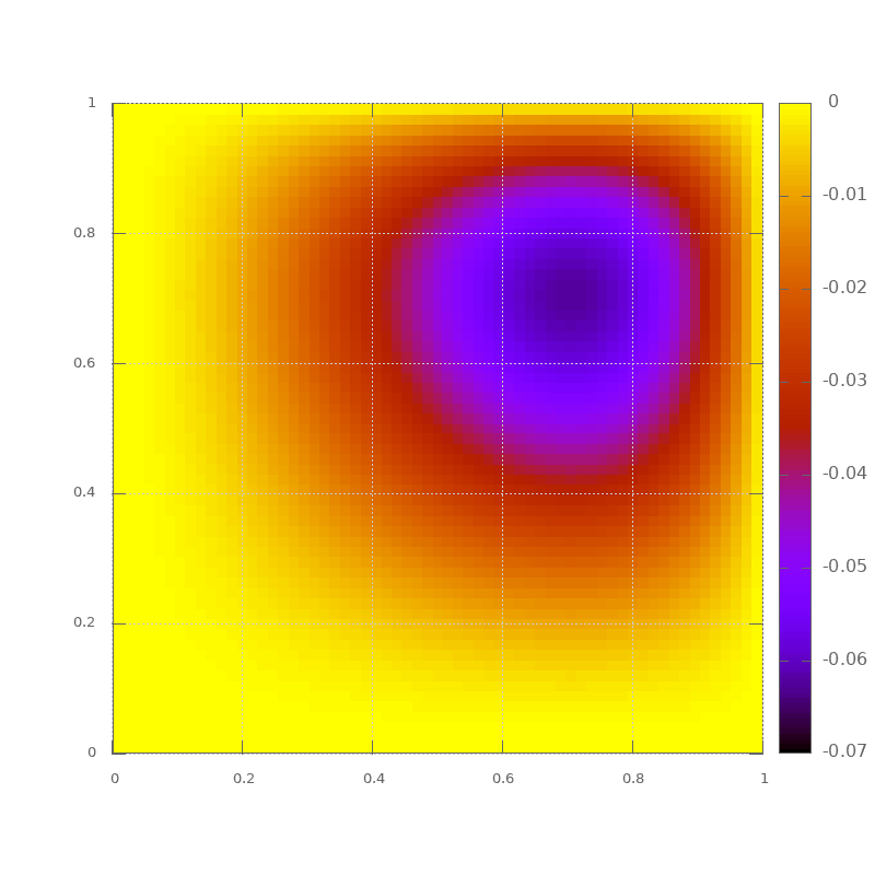
We’ll use this example next week when we do parallel programming.