Homework #7#
Completing this assignment
Upload your C++ source file (not the executables produced by g++) and the plot output (a PNG file) to Brightspace.
Important
Make sure your that g++ can compile your code. You
may need to use -std=c++20.
Important
All work must be your own.
You may not use generative AI / large-language models for any part of this assignment.
Projectiles with air-resistance :
Let’s try solving for projectile motion with drag (air resistance).
We want to solve:
\[\begin{split}\dot{\bf r} &= {\bf v} \\ \dot{\bf v} &= \frac{1}{m} {\bf F}_a({\bf v}) - |g| \hat{\bf y}\end{split}\]where \({\bf r} = (x, y)\) is the position vector, \({\bf v} = (v_x, v_y)\) is the velocity vector, \(m\) is the mass of the projectile and
\[{\bf F}_a({\bf v}) = - \frac{1}{2}C \rho_\mathrm{air} A |v| {\bf v}\]is the Newton drag term that is applicable for large Reynolds numbers (turbulent), and \(\rho_\mathrm{air}\) is the density of air, \(C\) is the drag coefficient, \(A\) is the cross-sectional area of the projectile.
Note
Gravity only affects the vertical (\(y\)) component of velocity, but drag affects both, since it is proportional to \({\bf v}\).
We’ll consider a baseball. Then we can take:
\(C = 0.3\)
\(A = \pi (d/2)^2\) with the diameter of a bassball, \(d = 0.074~\mathrm{m}\)
\(m = 0.145~\mathrm{kg}\)
\(\rho_\mathrm{air} = 1.2~\mathrm{kg~m^{-3}}\)
and we take the gravitational acceleration to be \(g = -9.81~\mathrm{m~s^{-2}}\),
We’ll imagine throwing the baseball from some height, \(y_0\), above the ground (\(y = 0\)) at an angle \(\theta\) from the horizontal with velocity magnitude \(v_0\).
This means our initial conditions are:
\[\begin{split}x_0 &= 0 \\ y_0 &= y_0 \\ {v_x}_0 &= v_0 \cos(\theta) \\ {v_y}_0 &= v_0 \sin(\theta)\end{split}\]and we want to integrate until the ball hits the ground, \(y(t_\mathrm{max}) = 0\).
Your task
Solve this system using our 2nd-order Runge-Kutta method.
You should structure your program the same way we did for our 2nd-order Runge-Kutta Orbit code in class. The main differences will be to the righthand side function and the stopping criterion.
Run the case with and without drag (you can set \(C = 0\) for no drag), and plot the results together on the same plot.
Tip
If you have 2 output files,
file1.txtandfile2.txt, you can plot both of them together in gnuplot as:plot 'file1.txt' using 1:2 title "no drag", 'file2.txt' using 1:2 title "drag"This will plot column 2 vs. column 1 from each file as separate lines and label them in the plot.
solution
Here’s the code:
#include <iostream>
#include <vector>
#include <cmath>
#include <numbers>
#include <format>

const double d = 0.074;
const double A = std::numbers::pi * d * d;
const double m = 0.145;
const double rho_air = 1.2;
const double g = -9.81;

struct OrbitState {
    double t;
    double x;
    double y;
    double vx;
    double vy;
};

OrbitState rhs(const OrbitState& state, double C) {

    OrbitState dodt{};

    // dx/dt = vx; dy/dt = vy

    dodt.x = state.vx;
    dodt.y = state.vy;

    // d(vx)/dt = - 1/2 C rho_air A |v| vx / m
    // d(vy)/dt = - 1/2 C rho_air A |v| vy / m - |g|

    double v = std::sqrt(state.vx * state.vx + state.vy * state.vy);

    dodt.vx = -0.5 * C * rho_air * A * v * state.vx / m;
    dodt.vy = -0.5 * C * rho_air * A * v * state.vy / m - std::abs(g);

    return dodt;

}

OrbitState update_state(const OrbitState& state,
                        const double dt,
                        const OrbitState& state_derivs) {

    OrbitState state_new{};

    state_new.t = state.t + dt;
    state_new.x = state.x + dt * state_derivs.x;
    state_new.y = state.y + dt * state_derivs.y;
    state_new.vx = state.vx + dt * state_derivs.vx;
    state_new.vy = state.vy + dt * state_derivs.vy;

    return state_new;
}

void write_history(const std::vector<OrbitState>& history) {

    for (const auto& o : history) {
        std::cout
            << std::format("{:11.8f} {:11.8f} {:11.8f} {:11.8f} {:11.8f}\n",
                           o.t, o.x, o.y, o.vx, o.vy);
    }
}

std::vector<OrbitState> integrate(const OrbitState& state0,
                                  const double C,
                                  const double dt_in) {

    // how the history of the orbit

    std::vector<OrbitState> orbit_history{};
    orbit_history.push_back(state0);

    double dt = dt_in;

    OrbitState state = state0;

    // integration loop
    while (state.y > 0.0) {

        // get the derivatives
        auto state_derivs = rhs(state, C);

        // get the derivatives at the midpoint in time
        auto state_star = update_state(state, 0.5 * dt, state_derivs);
        state_derivs = rhs(state_star, C);

        // update the state
        state = update_state(state, dt, state_derivs);

        orbit_history.push_back(state);
    }

    return orbit_history;

}

int main() {

    // set initial conditions
    OrbitState state0{};

    double C{};
    std::cout << "# Enter the drag coefficient C: ";
    std::cin >> C;
    std::cout << std::endl;

    // initial velocity and angle
    double v0 = 10.0;
    double theta = std::numbers::pi / 4.0;

    // initial height
    double y0 = 10.0;

    state0.t = 0.0;
    state0.x = 0.0;
    state0.y = y0;
    state0.vx = v0 * std::cos(theta);
    state0.vy = v0 * std::sin(theta);

    double dt = 0.05;

    auto orbit_history = integrate(state0, C, dt);
    write_history(orbit_history);

}
Notice that our while loop is:
while (state.y > 0.0) {
    ...
}
This will keep looping until the projectile hits the ground.
This prompts the user for the drag coefficient when run. You can run both cases as:
echo 0.0 | ./projectile > proj-nodrag.txt echo 0.3 | ./projectile > proj-drag0.3.txt
Note
It’s fine also if you just hardcode the value of \(C\) into the program and recompile each time.
To make the plot, given the output names above, we can use this GNUplot script:
set term png enhanced size 800,600
set output "projectile-drag.png"

set xlabel "x"

set ylabel "y"
set yrange [0:]

set grid

plot 'proj-nodrag.txt' using 2:3 title "no drag", \
     'proj-drag0.3.txt' using 2:3 title "C = 0.3"
which produces this image:
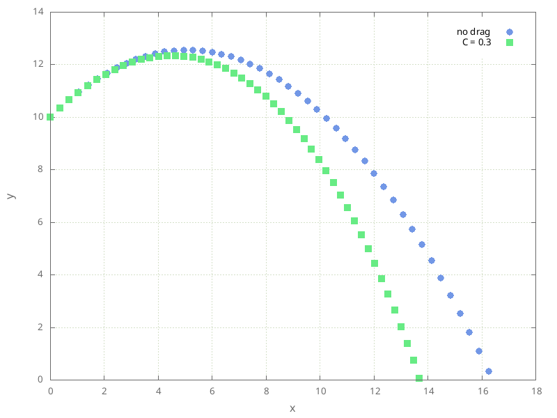
Fig. 16 The motion of the projectile with and without drag.#