Example: Planetary Orbit

Let’s consider an example of integrating the orbit of Earth around the Sun (we’ll consider the mass of the Earth to be tiny compared to the Sun so we can neglect the Sun’s motion around the center of mass).

Kepler’s third law tells us:

\[4\pi^2 a^3 = G M_\star P^2\]

where \(a\) is the semi-major axis and \(P\) is the period of the orbit. If we work in units of solar masses, astronomical units, and years, then this becomes:

\[a^3 = P^2\]

which implies that \(G M_\star = 4 \pi^2\).

The evolution of the planet is given by

\[\dot{\bf r} = {\bf v}\]

\[\dot{\bf v} = - \frac{G M_\star {\bf r}}{r^3}\]

where \({\bf r} = (x, y)\) and \({\bf v} = (v_x, v_y)\) are vectors. This means that we have 4 equations overall to advance.

Note

We use \(\dot{y}\) as our notation for a time-derivative, \(dy/dt\),

Important

This is 4 first-order ordinary differential equations, so we need 4 initial conditions.

We want to evolve the orbit of Earth around the Sun using these ODEs.

Euler’s Method

Using Euler’s method, as we just learned, the solution begins with a first-order accurate difference approximation to the derivative:

\[\frac{{\bf r}^{n+1} - {\bf r}^n}{\tau} = {\bf v}^n + \mathcal{O}(\tau)\]

\[\frac{{\bf v}^{n+1} - {\bf v}^n}{\tau} = {\bf a}({\bf r}^n,{\bf v}^n) + \mathcal{O}(\tau)\]

or

\[{\bf r}^{n+1} = {\bf r}^n + \tau {\bf v}^n + \mathcal{O}(\tau^2)\]

\[{\bf v}^{n+1} = {\bf v}^n + \tau {\bf a}({\bf r}^n,{\bf v}^n) + \mathcal{O}(\tau^2)\]

Implementation

We’ll store the state of the solution at a single instance in time in a struct:

struct OrbitState {
    double t;
    double x;
    double y;
    double vx;
    double vy;
};

and we’ll save the solution at each step in a vector:

std::vector<OrbitState> orbit_history{};

This corresponds to the “array-of-structs” storage scheme we discussed in our Vector of Structs section.

To make our code flexible, we’ll write the following functions:

• A righthand side function, that takes an OrbitState and returns an OrbitState:

  OrbitState rhs(const OrbitState& state);
  

  We can compute all of the ODE righthand sides from the input state and then return the derivatives using an OrbitState (there, each component will actually be the derivative in time).

  As we’ve seen a few times now, we pass this in as a const reference for performance. The const ensures that it is read-only.

• A function to write out the history:

  void write_history(const std::vector<OrbitState>& history);
  

  We can adapt this as desired to write to the screen or a file (which we’ll see soon).

• An integration function:

  std::vector<OrbitState> integrate(const double a,
                                    const double tmax, const double dt);
  

  This manages the time-stepping, implementing Euler’s method and storing the solution in our history vector each step. At the end of integration it will return the history.

  An important parameter here is dt—the size of our timestep. We’ll see that it has a large influence on the quality of our solution.

Implementation

Here’s our implementation:

Listing 71 orbit_example.cpp

#include <iostream>
#include <iomanip>
#include <vector>
#include <cmath>
#include <numbers>
#include <format>

// G * Mass in AU, year, solar mass units
const double GM = 4.0 * std::numbers::pi * std::numbers::pi;

struct OrbitState {
    double t;
    double x;
    double y;
    double vx;
    double vy;
};

OrbitState rhs(const OrbitState& state) {

    OrbitState dodt{};

    // dx/dt = vx; dy/dt = vy

    dodt.x = state.vx;
    dodt.y = state.vy;

    // d(vx)/dt = - GMx/r**3; d(vy)/dt = - GMy/r**3

    double r = std::sqrt(state.x * state.x + state.y * state.y);

    dodt.vx = - GM * state.x / std::pow(r, 3);
    dodt.vy = - GM * state.y / std::pow(r, 3);

    return dodt;

}

void write_history(const std::vector<OrbitState>& history) {

    for (const auto& o : history) {
        std::cout
            << std::format("{:11.8f} {:11.8f} {:11.8f} {:11.8f} {:11.8f}\n",
                           o.t, o.x, o.y, o.vx, o.vy);
    }
}

std::vector<OrbitState> integrate(const double a,
                                  const double tmax,
                                  const double dt_in) {

    // how the history of the orbit

    std::vector<OrbitState> orbit_history{};

    // set initial conditions
    OrbitState state{};

    // assume circular orbit on the x-axis, counter-clockwise orbit

    state.t = 0.0;
    state.x = a;
    state.y = 0.0;
    state.vx = 0.0;
    state.vy = std::sqrt(GM / a);

    orbit_history.push_back(state);

    double dt = dt_in;

    // integration loop
    while (state.t < tmax) {

        // if the final dt step takes us past our stopping time
        // (tmax), cut the timestep
        if (state.t + dt > tmax) {
            dt = tmax - state.t;
        }

        // get the derivatives
        auto state_derivs = rhs(state);

        // update the state
        state.t += dt;
        state.x += state_derivs.x * dt;
        state.y += state_derivs.y * dt;
        state.vx += state_derivs.vx * dt;
        state.vy += state_derivs.vy * dt;

        orbit_history.push_back(state);
    }

    return orbit_history;

}

int main() {

    double tmax = 1.0;
    double dt = 0.05;
    double a = 1.0;      // 1 AU

    auto orbit_history = integrate(a, tmax, dt);
    write_history(orbit_history);

}

Some notes:

• We make GM a const, since it should not change.

• In our integrate function, we create an OrbitState named state. This will hold the current state at the start of each step / loop iteration, and be advanced to the new time at the end of the loop iteration.

  Note that when we do:

  orbit_history.push_back(state);
  

  We are making a copy of state and storing it in our orbit_history vector.

• We have a check to ensure that the last step does not take us past the maximum time we want to evolve for:

  if (state.t + dt > tmax) {
      dt = tmax - state.t;
  }
  

Running

This is setup for Earth (the semi-major axis is 1 AU), and to integrate for 1 year. After this time, the Earth should be right back where it started. Any difference in the final position from the initial position is integration error.

From our method, we expect that the error will decrease by a factor of 2 each time we cut the timestep in half.

We control is the timestep. Our default, dt = 0.05 corresponds to 1/20th of a year. The main question is—how small does our timestep need to be to get an acceptable solution?

Plotting

We can plot the solution using gnuplot.

First, when you run, redirect the output to a file:

./orbit_example > orbit.dat

Now run gnuplot:

gnuplot

Again, we’ll use plot and plot different columns against one another:

set size ratio -1
set xlabel "x"
set ylabel "y"
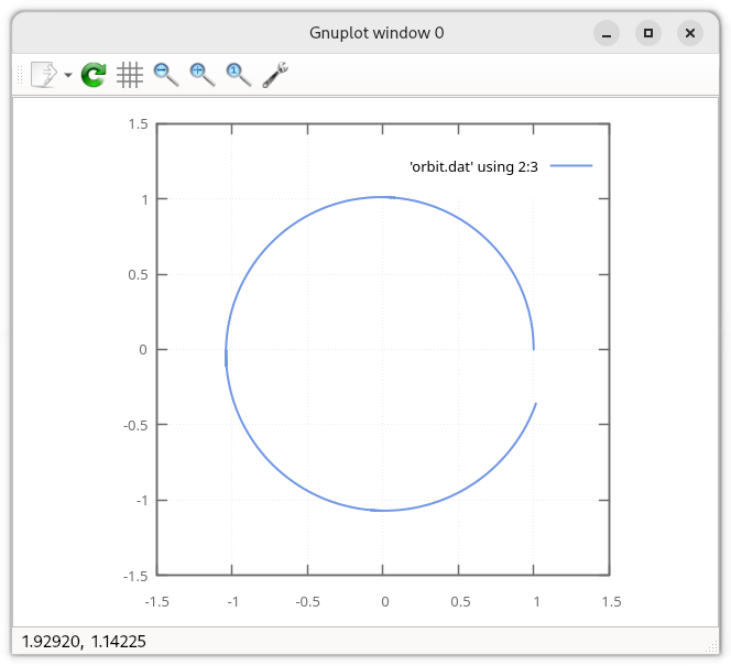
plot 'orbit.dat' using 2:3 notitle w l

This will make something like:

Tip

We used a new gnuplot command here:

set size ratio -1

This ensures that the aspect ratio of the coordinates is preserved (so a circle will appear as a circle in our plot).

You can save the plot as:

set term png enhanced
set output "orbit.png"
replot

Look how bad this is!!!

We should have a nice circular orbit, but it goes way off a circle and out to much greater distances in the solar system.

The problem here is that our timestep is too large—truncation error is dominating.

try it…

Let’s see how the solution behaves as we cut the timestep.