2nd-order Runge-Kutta Orbit

The main utility of functions is that we can reuse them in a code. Let’s look at this by extending our Euler integration of an orbit to do 2nd-order Runge-Kutta integration.

The Euler method was based on a first-order difference approximation to the derivative. But a centered-difference approximation to \(df/dt\) is second order accurate at the midpoint in time, so we can try to update our system in the form:

\[\frac{{\bf r}^{n+1} - {\bf r}^n}{\tau} = {\bf v}^{n+1/2} + \mathcal{O}(\tau^2)\]

\[\frac{{\bf v}^{n+1} - {\bf v}^n}{\tau} = {\bf a}^{n+1/2} + \mathcal{O}(\tau^2)\]

Then the updates are:

\[{\bf r}^{n+1} = {\bf r}^n + \tau \, {\bf v}^{n+1/2} + \mathcal{O}(\tau^3)\]

\[{\bf v}^{n+1} = {\bf v}^n + \tau \, {\bf a}^{n+1/2} + \mathcal{O}(\tau^3)\]

This is locally third-order accurate (but globally second-order accurate), but we don’t know how to compute the state at the half-time.

To find the \(n+1/2\) state, we first use Euler’s method to predict the state at the midpoint in time. We then use this provisional state to evaluate the accelerations at the midpoint and use those to update the state fully through \(\tau\).

The two step process appears as:

\[{\bf r}^\star = {\bf r}^n + (\tau / 2) {\bf v}^n\]

\[{\bf v}^\star = {\bf v}^n + (\tau / 2) {\bf a}^n\]

then we use this for the full update:

\[{\bf r}^{n+1} = {\bf r}^n + \tau \, {\bf v}^\star\]

\[{\bf v}^{n+1} = {\bf v}^n + \tau \, {\bf a}({\bf r}^\star)\]

Graphically this looks like the following:

First we take a half step and we evaluate the slope at the midpoint:

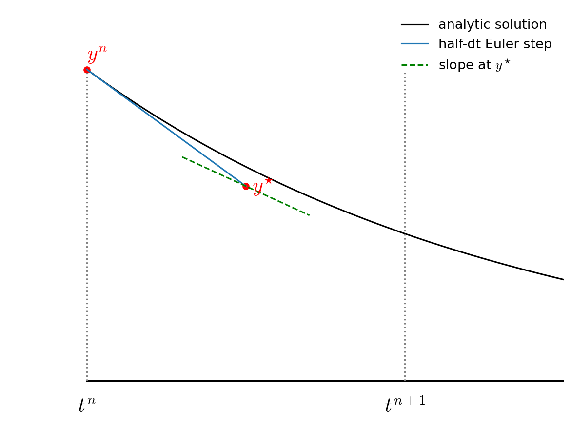
Fig. 8 The predictor part of RK2 integration.

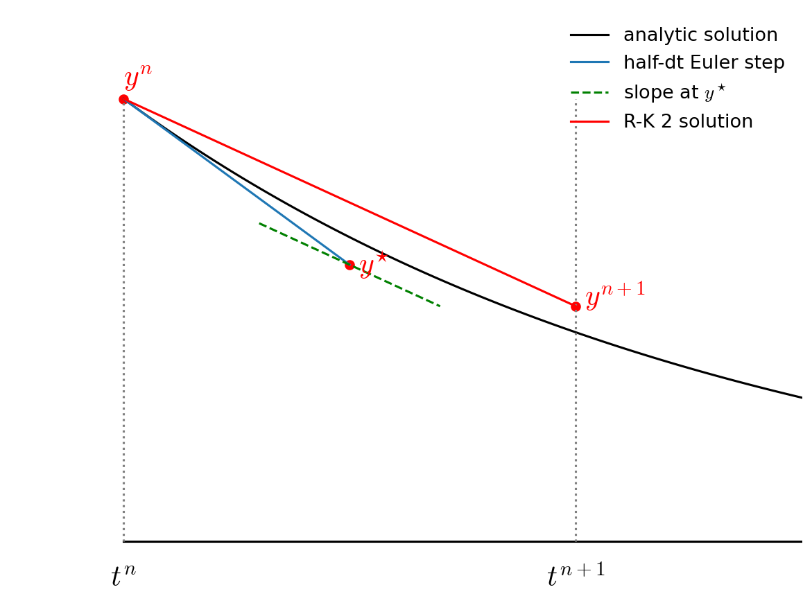
Fig. 9 The corrector / final update of RK2 integration.

Notice how the final step (the red line) is parallel to the slope we computed at \(t^{n+1/2}\). Also note that the solution at \(t^{n+1}\) is much closer to the analytic solution than in the figure from Euler’s method.

This method is called 2nd-order Runge-Kutta.

Implementation

To implement this, it would be nice to have a function that updates the state based on the derivatives, like:

OrbitState update_state(const OrbitState& state, const double dt,
                        const OrbitState& state_derivs);

This way we can easily do the update both times as needed via a simple function call.

Tip

Later we’ll learn how to use operator overloading to do something like:

OrbitState state{};
double dt{};
OrbitState state_derivs{};

...

auto state_new = state + dt * state_derivs;

Our implementation looks largely the same as the first-order method:

Listing 72 orbit_rk2_example.cpp

#include <iostream>
#include <iomanip>
#include <vector>
#include <cmath>
#include <numbers>
#include <format>

// G * Mass in AU, year, solar mass units
const double GM = 4.0 * std::numbers::pi * std::numbers::pi;

struct OrbitState {
    double t;
    double x;
    double y;
    double vx;
    double vy;
};

OrbitState rhs(const OrbitState& state) {

    OrbitState dodt{};

    // dx/dt = vx; dy/dt = vy

    dodt.x = state.vx;
    dodt.y = state.vy;

    // d(vx)/dt = - GMx/r**3; d(vy)/dt = - GMy/r**3

    double r = std::sqrt(state.x * state.x + state.y * state.y);

    dodt.vx = - GM * state.x / std::pow(r, 3);
    dodt.vy = - GM * state.y / std::pow(r, 3);

    return dodt;

}

OrbitState update_state(const OrbitState& state,
                        const double dt,
                        const OrbitState& state_derivs) {

    OrbitState state_new{};

    state_new.t = state.t + dt;
    state_new.x = state.x + dt * state_derivs.x;
    state_new.y = state.y + dt * state_derivs.y;
    state_new.vx = state.vx + dt * state_derivs.vx;
    state_new.vy = state.vy + dt * state_derivs.vy;

    return state_new;
}

void write_history(const std::vector<OrbitState>& history) {

    for (const auto& o : history) {
        std::cout
            << std::format("{:11.8f} {:11.8f} {:11.8f} {:11.8f} {:11.8f}\n",
                           o.t, o.x, o.y, o.vx, o.vy);
    }
}

std::vector<OrbitState> integrate(const double a,
                                  const double tmax,
                                  const double dt_in) {

    // how the history of the orbit

    std::vector<OrbitState> orbit_history{};

    // set initial conditions
    OrbitState state{};

    // assume circular orbit on the x-axis, counter-clockwise orbit

    state.t = 0.0;
    state.x = a;
    state.y = 0.0;
    state.vx = 0.0;
    state.vy = std::sqrt(GM / a);

    orbit_history.push_back(state);

    double dt = dt_in;

    // integration loop
    while (state.t < tmax) {

        // if the final dt step takes us past our stopping time
        // (tmax), cut the timestep
        if (state.t + dt > tmax) {
            dt = tmax - state.t;
        }

        // get the derivatives
        auto state_derivs = rhs(state);

        // get the derivatives at the midpoint in time
        auto state_star = update_state(state, 0.5 * dt, state_derivs);
        state_derivs = rhs(state_star);

        // update the state
        state = update_state(state, dt, state_derivs);

        orbit_history.push_back(state);
    }

    return orbit_history;

}

int main() {

    double tmax = 1.0;
    double dt = 0.05;
    double a = 1.0;      // 1 AU

    auto orbit_history = integrate(a, tmax, dt);
    write_history(orbit_history);

}

The main difference is that we compute an intermediate solution at the half-time:

// get the derivatives at the midpoint in time
auto state_star = update_state(state, 0.5 * dt, state_derivs);
state_derivs = rhs(state_star);

This makes the final update time-centered, and gives us second-order accuracy.

When run with dt = 0.05, we get:

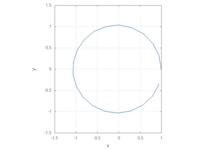
We see that this is far better than the first-order Euler method. It is still not perfect, but as we cut the timestep, the solution should improve much faster than the Euler case.

Error estimate

We can estimate the error by computing the initial distance from the Sun and comparing to the final distance from the Sun. The orbit is circular, so it should be constant.

try it…

Let’s write an error function of the form:

double error(const std::vector<OrbitState>& history)

that computes this error, and the output the error at the end of integration for a variety of timestep sizes.

solution

Here’s a version of the code with the error function and a loop in the main function that explores different timestep sizes.

Listing 73 orbit_rk2_error.cpp

#include <iostream>
#include <iomanip>
#include <vector>
#include <cmath>
#include <numbers>
#include <format>

// G * Mass in AU, year, solar mass units
const double GM = 4.0 * std::numbers::pi * std::numbers::pi;

struct OrbitState {
    double t;
    double x;
    double y;
    double vx;
    double vy;
};

OrbitState rhs(const OrbitState& state) {

    OrbitState dodt{};

    // dx/dt = vx; dy/dt = vy

    dodt.x = state.vx;
    dodt.y = state.vy;

    // d(vx)/dt = - GMx/r**3; d(vy)/dt = - GMy/r**3

    double r = std::sqrt(state.x * state.x + state.y * state.y);

    dodt.vx = - GM * state.x / std::pow(r, 3);
    dodt.vy = - GM * state.y / std::pow(r, 3);

    return dodt;

}

OrbitState update_state(const OrbitState& state,
                        const double dt,
                        const OrbitState& state_derivs) {

    OrbitState state_new{};

    state_new.t = state.t + dt;
    state_new.x = state.x + dt * state_derivs.x;
    state_new.y = state.y + dt * state_derivs.y;
    state_new.vx = state.vx + dt * state_derivs.vx;
    state_new.vy = state.vy + dt * state_derivs.vy;

    return state_new;
}

double error(const std::vector<OrbitState>& history) {

    // compute the orbital radius at the start and end of integration
    double R_start = std::sqrt(std::pow(history[0].x, 2.0) +
                               std::pow(history[0].y, 2.0));

    auto idx_end = history.size() - 1;
    double R_end = std::sqrt(std::pow(history[idx_end].x, 2.0) +
                             std::pow(history[idx_end].y, 2.0));

    return std::abs(R_start - R_end);

}

std::vector<OrbitState> integrate(const double a,
                                  const double tmax,
                                  const double dt_in) {

    // how the history of the orbit

    std::vector<OrbitState> orbit_history{};

    // set initial conditions
    OrbitState state{};

    // assume circular orbit on the x-axis, counter-clockwise orbit

    state.t = 0.0;
    state.x = a;
    state.y = 0.0;
    state.vx = 0.0;
    state.vy = std::sqrt(GM / a);

    orbit_history.push_back(state);

    double dt = dt_in;

    // integration loop
    while (state.t < tmax) {

        // if the final dt step takes us past our stopping time
        // (tmax), cut the timestep
        if (state.t + dt > tmax) {
            dt = tmax - state.t;
        }

        // get the derivatives
        auto state_derivs = rhs(state);

        // get the derivatives at the midpoint in time
        auto state_star = update_state(state, 0.5 * dt, state_derivs);
        state_derivs = rhs(state_star);

        // update the state
        state = update_state(state, dt, state_derivs);

        orbit_history.push_back(state);
    }

    return orbit_history;

}

int main() {

    double tmax = 1.0;
    double a = 1.0;

    // consider several different timesteps and output the error
    for (auto dt : {0.1, 0.05, 0.025, 0.0125, 0.00625}) {
        auto orbit_history = integrate(a, tmax, dt);
        auto err = error(orbit_history);
        std::cout << std::format("{:7.5f} {:12.6g}\n", dt, err);
    }

}

When this is run, we get:

0.10000    0.0116001
0.05000    0.0111227
0.02500   0.00247085
0.01250  0.000360686
0.00625  4.69261e-05

For very coarse dt, we have a large error, but once dt is below 0.05, we see that the solution is converging 2nd-order or better.

Note

Comparing the starting and ending radius is just one error measure. We could also consider the distance between the initial and final positions or the total energy of the system. Each of these should converge 2nd order once the timestep is small enough.