Ordinary Differential Equations

Consider an ordinary differential equation,

\[\frac{dy}{dt} = f(y)\]

To solve this we need some initial conditions, \(y(t = 0) = 0\).

Note

We’ll use \(\dot{y}\) as our notation for a time-derivative, \(dy/dt\), so we can write our system as:

\[\dot{y} = f(y)\]

To advance this system, we can use a finite difference approximation for the time-derivative:

\[\frac{y^{n+1} - y^n}{\tau} = f(y^n)\]

where \(y^n\) means \(y(t = t^n)\) and \(y^{n+1}\) means \(y(t = t^n + \tau)\) where \(\tau\) is the timestep that we use to advance the system.

To evolve the system for a long time, we take many steps of size \(\tau\).

The new solution is then:

\[y^{n+1} = y^n + \tau f(y^n) + \mathcal{O}(\tau^2)\]

This method is called Euler’s method.

This shows that each time we take a step, we make an error (called truncation error) of \(\mathcal{O}(\tau^2)\). Over the course of the orbit we will take \(N = T / \tau\) steps, so the global error will be \(\mathcal{O}(\tau)\).

Visually, our method looks like:

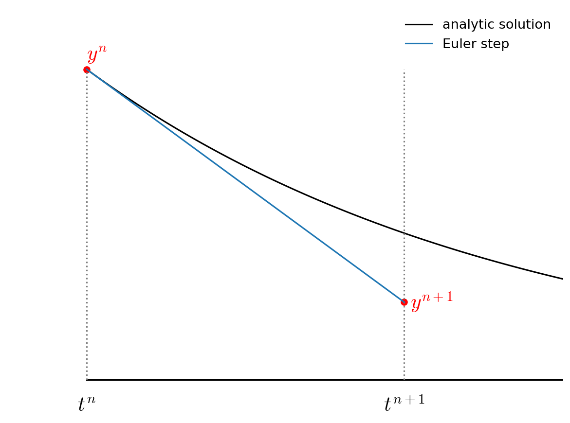
We evaluate the derivative at the start of the timestep and follow that slope to the new time. As shown in the figure, the error in this method is the difference between the true solution (black line) and the data point at the new time, \(y^{n+1}\).