4th-order Runge-Kutta

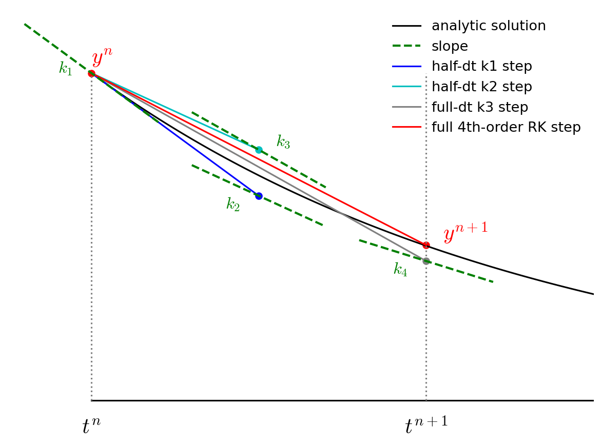
One of the most widely-used methods for ODE integration is 4th-order Runge-Kutta (RK4). This consists of 4 stages, each estimating the slope of the solution at a different time or with a different prediction of the state. These are then combined in a final update to advance the solution. The sequence is illustrated below:

Stage 1

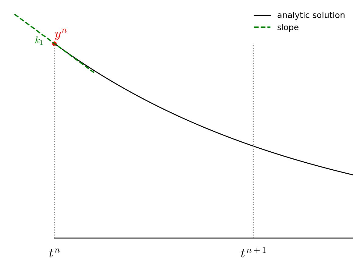
The advance begins by estimating the derivatives (righthand side or slope) at time \(t^n\). We’ll call this \({\bf k}_1\).

\[{\bf k}_1 = {\bf f}(t^n, {\bf y}^n)\]

Stage 2

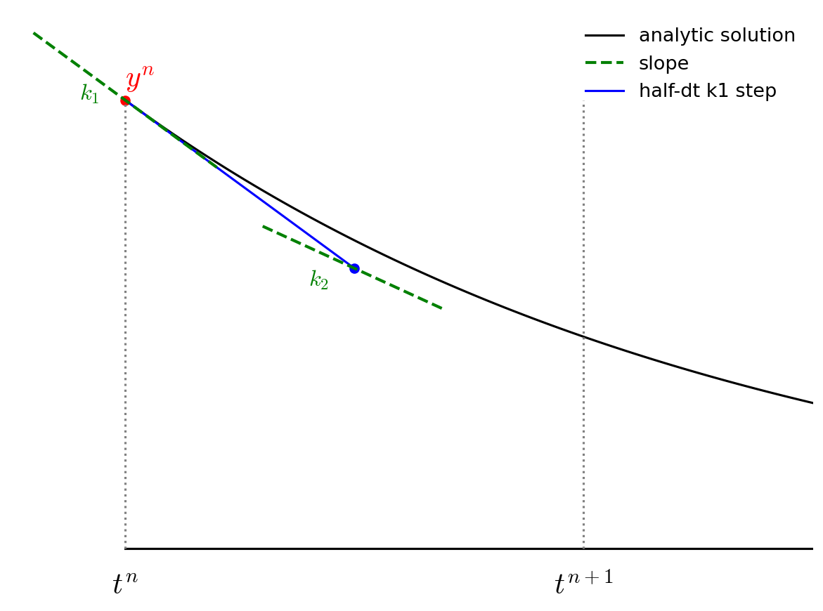
We then follow the slope \({\bf k}_1\) to the midpoint in time, \(t^{n+1/2}\) and evaluate the slope there. We call the new slope \({\bf k}_2\).

\[{\bf k}_2 = {\bf f}(t^n + \tau/2, {\bf y}^n + (\tau/2) {\bf k}_1)\]

Stage 3

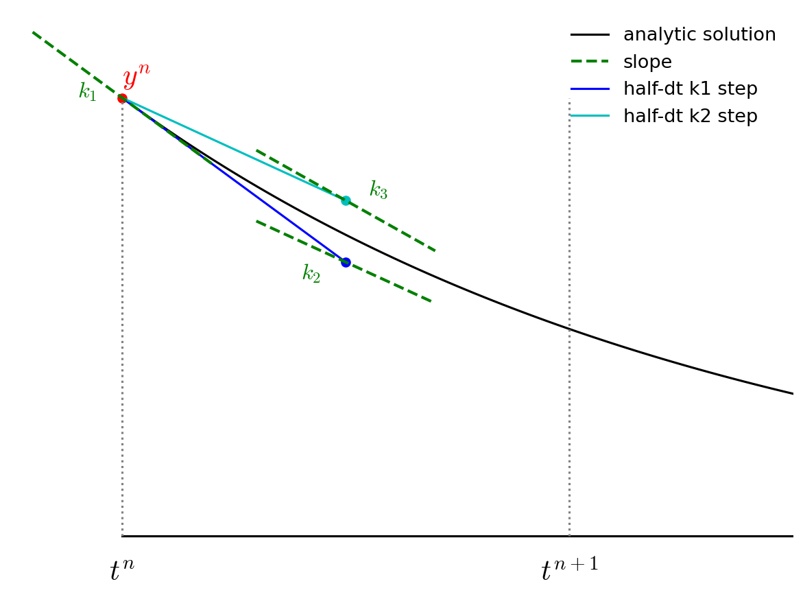
We then go back to the start, but this time follow the new slope, \({\bf k}_2\) to the midpoint in time, \(t^{n+1/2}\). We again evaluate the slope here, and call it \({\bf k}_3\).

\[{\bf k}_3 = {\bf f}(t^n + \tau/2, {\bf y}^n + (\tau/2) {\bf k}_2)\]

Stage 4

Finally, we go back to the start and follow \({\bf k}_3\) for the full timestep, to \(t^{n+1}\) and evaluate the slope there, calling it \({\bf k}_4\).

\[{\bf k}_4 = {\bf f}(t^n + \tau, {\bf y}^n + \tau {\bf k}_3)\]

Final update

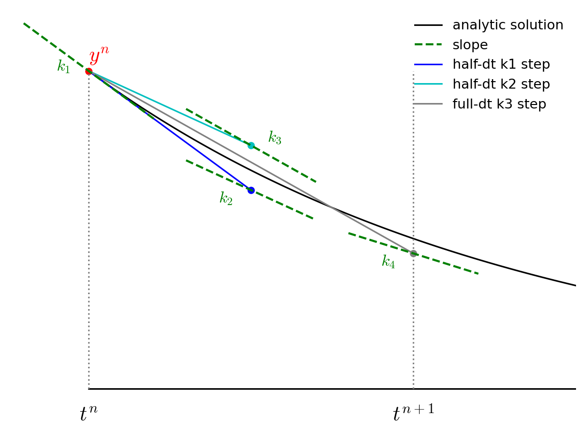
We then get the updated solution using a linear combination of the 4 slopes:

\[{\bf y}^{n+1} = {\bf y}^n + \frac{\tau}{6} ({\bf k}_1 + 2 {\bf k}_2 + 2 {\bf k}_3 + {\bf k}_4)\]

Note the similarity of RK4 to Simpson’s rule for integration.

try it…

Let’s modify our orbit integration code to do RK4.

solution

Listing 74 orbit_rk4_error.cpp

#include <iostream>
#include <iomanip>
#include <vector>
#include <cmath>
#include <numbers>
#include <format>

// G * Mass in AU, year, solar mass units
const double GM = 4.0 * std::numbers::pi * std::numbers::pi;

struct OrbitState {
    double t;
    double x;
    double y;
    double vx;
    double vy;
};

OrbitState rhs(const OrbitState& state) {

    OrbitState dodt{};

    // dx/dt = vx; dy/dt = vy

    dodt.x = state.vx;
    dodt.y = state.vy;

    // d(vx)/dt = - GMx/r**3; d(vy)/dt = - GMy/r**3

    double r = std::sqrt(state.x * state.x + state.y * state.y);

    dodt.vx = - GM * state.x / std::pow(r, 3);
    dodt.vy = - GM * state.y / std::pow(r, 3);

    return dodt;

}

OrbitState update_state(const OrbitState& state,
                        const double dt,
                        const OrbitState& state_derivs) {

    OrbitState state_new{};

    state_new.t = state.t + dt;
    state_new.x = state.x + dt * state_derivs.x;
    state_new.y = state.y + dt * state_derivs.y;
    state_new.vx = state.vx + dt * state_derivs.vx;
    state_new.vy = state.vy + dt * state_derivs.vy;

    return state_new;
}

double error(const std::vector<OrbitState>& history) {

    // compute the orbital radius at the start and end of integration
    double R_start = std::sqrt(std::pow(history[0].x, 2.0) +
                               std::pow(history[0].y, 2.0));

    auto idx_end = history.size() - 1;
    double R_end = std::sqrt(std::pow(history[idx_end].x, 2.0) +
                             std::pow(history[idx_end].y, 2.0));

    return std::abs(R_start - R_end);

}

std::vector<OrbitState> integrate(const double a,
                                  const double tmax,
                                  const double dt_in) {

    // how the history of the orbit

    std::vector<OrbitState> orbit_history{};

    // set initial conditions
    OrbitState state{};

    // assume circular orbit on the x-axis, counter-clockwise orbit

    state.t = 0.0;
    state.x = a;
    state.y = 0.0;
    state.vx = 0.0;
    state.vy = std::sqrt(GM / a);

    orbit_history.push_back(state);

    double dt = dt_in;

    // integration loop
    while (state.t < tmax) {

        // if the final dt step takes us past our stopping time
        // (tmax), cut the timestep
        if (state.t + dt > tmax) {
            dt = tmax - state.t;
        }

        // get the derivatives
        auto k1 = rhs(state);

        // get the derivatives at the midpoint in time
        auto state_star = update_state(state, 0.5 * dt, k1);
        auto k2 = rhs(state_star);

        state_star = update_state(state, 0.5 * dt, k2);
        auto k3 = rhs(state_star);

        state_star = update_state(state, dt, k3);
        auto k4 = rhs(state_star);

        // update the state
        state.t += dt;
        state.x += dt / 6.0 * (k1.x + 2.0 * k2.x + 2.0 * k3.x + k4.x);
        state.y += dt / 6.0 * (k1.y + 2.0 * k2.y + 2.0 * k3.y + k4.y);
        state.vx += dt / 6.0 * (k1.vx + 2.0 * k2.vx + 2.0 * k3.vx + k4.vx);
        state.vy += dt / 6.0 * (k1.vy + 2.0 * k2.vy + 2.0 * k3.vy + k4.vy);

        orbit_history.push_back(state);
    }

    return orbit_history;

}

int main() {

    double tmax = 1.0;
    double a = 1.0;

    // consider several different timesteps and output the error
    for (auto dt : {0.1, 0.05, 0.025, 0.0125, 0.00625}) {
        auto orbit_history = integrate(a, tmax, dt);
        auto err = error(orbit_history);
        std::cout << std::format("{:7.5f} {:12.6g}\n", dt, err);
    }

}

When run, we see the convergence as:

0.10000    0.0202442
0.05000  0.000547327
0.02500  1.67785e-05
0.01250  5.22248e-07
0.00625  1.63047e-08