Integration

In calculus, you saw a definition of a definite integral that looked something like:

\[I \equiv \int_a^b f(x) dx = \lim_{\Delta x \rightarrow 0} \sum_{i = 1}^N f(x_i) \Delta x\]

where the number of intervals you divide \([a, b]\) into, \(N\), is defined such that \(N = (b -a) / \Delta x\).

Also recall that this definition is directly related to the interpretation of an integral representing the area under a curve.

Rectangle rule

The simplest way to compute the integral is to treat each interval as a rectangle:

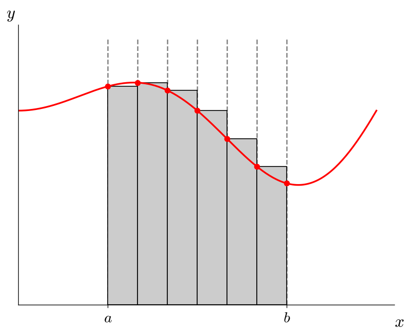
Fig. 6 The rectangle rule—we divide the area under the curve into intervals (\(N = 6\) shown here) and represent each as a rectangle.

Adding up the area of each rectangle, we have an approximation to the integral:

\[\int_a^b f(x) dx = {\Delta x} \sum_{i=0}^{N-1} f_i + \mathcal{O}(\Delta x)\]

This is not very accurate, and the truncation error can be shown to be \(\mathcal{O}(\Delta x)\)—making the method first-order accurate.

Trapezoid rule

The trapezoid rule is an improvement on the rectangle rule. Now we use the function values on the left and right edges of each interval (\(f_l\) and \(f_r\) respectively) and connect them with a line. This makes the area in each interval a trapezoid, with an area of \(\frac{1}{2}\Delta x (f_l + f_r)\).

Visually this appears as:

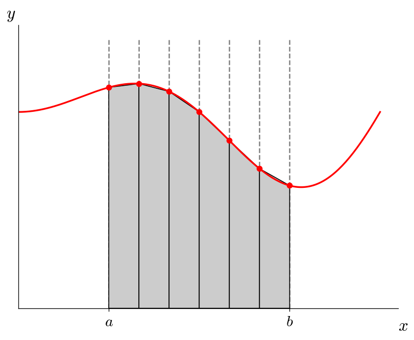
Fig. 7 The trapezoid rule—again using \(N = 6\), we connect the left and right function values for each interval, making trapezoids.

Summing the areas over all the intervals, we get an approximation for the integral:

\[\int_a^b f(x) dx = \frac{\Delta x}{2} \sum_{i=0}^{N-1} (f_i + f_{i+1}) + \mathcal{O}(\Delta x^2)\]

This is second-order accurate, and usually works quite well.

Example

Let’s try out the trapezoid rule with the function:

\[f(x) = 1 + \frac{x}{4} \sin(\pi x)\]

on the interval \([1/2, 3/2]\).

The analytic result is

\[I = 1 - \frac{1}{2\pi^2} \approx 0.949\]

Here’s an implementation that tries several different values of \(N\):

Listing 67 trapezoid.cpp

#include <iostream>
#include <functional>
#include <numbers>
#include <cmath>
#include <format>

double f(double x) {
    return 1.0 + 0.25 * x * std::sin(std::numbers::pi * x);
}


double I_analytic() {
    return 1.0 - 1.0 / (2.0 * std::pow(std::numbers::pi, 2.0));
}

double trapezoid(double a, double b, int N,
                 std::function<double(double)> func) {

    double dx = (b - a) / static_cast<int>(N);

    double I{};

    // loop over intervals
    for (int n = 0; n < N; ++n) {
        double xl = a + dx * n;
        double xr = a + dx * (n+1);

        double fl = func(xl);
        double fr = func(xr);

        I += 0.5 * dx * (fl + fr);
    }

    return I;

}


int main() {

    // perform trapezoid integration on f(x) for a variety on N and
    // compute the error compared to the analytic solution

    double a = 0.5;
    double b = 1.5;

    std::cout << std::format("{:^3} {:^10} {:^12}\n",
                             "N", "I", "error");

    for (auto N : {2, 4, 8, 16, 32, 64, 128}) {
        auto I = trapezoid(a, b, N, f);
        auto I_exact = I_analytic();
        double err = std::abs(I - I_exact);

        std::cout << std::format("{:3} {:10.5f} {:12.5e}\n",
                                 N, I, err);
    }
}

when run, we get:

 N      I         error
  2    0.93750  1.18394e-02
  4    0.94665  2.68650e-03
  8    0.94868  6.56092e-04
 16    0.94918  1.63075e-04
 32    0.94930  4.07097e-05
 64    0.94933  1.01738e-05
128    0.94934  2.54321e-06

Notice that we converge as second-order—as we double the number of intervals, the error goes down by \(4\times\).

try it…

Our code is a bit inefficient. We are computing the left and right function values each time in the loop. But the right function value for interval \(n\) becomes the left function value for interval \(n+1\). Let’s reuse these values in our loop, which will cut the number of function evaluations in half.