High-order Integration: Simpson’s Rule

One of the most popular methods of numerical integration is Simpson’s rule.

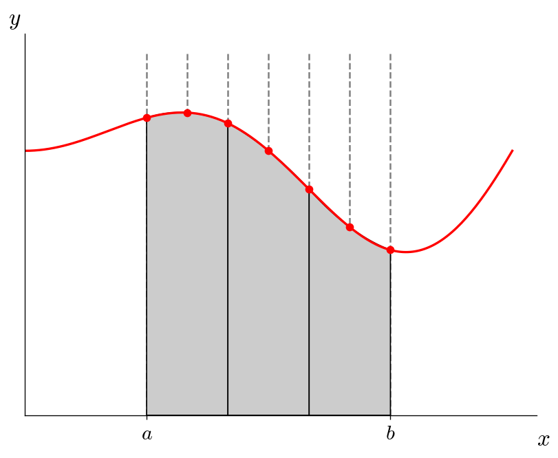
In the rectangle rule we used a constant in each interval. In the trapezoid rule, we used a line. In Simpson’s rule, we use a parabola. Since we need 3 points for a parabola, we need to use 2 intervals at a time.

Visually, this appears as:

Derivation

To derive Simpson’s rule, we would choose a parabola of the form:

\[f(x) = a (x - x_0)^2 + b (x - x_0) + c\]

and we fit it to 3 points: \((x_0, f_0)\), \((x_1, f_1)\), \((x_2, f_2)\), where we assume that these are equally spaced, \(x_1 = x_0 + \Delta x\) and \(x_2 = x_1 + \Delta x\).

Then evaluating it at the 3 points we have:

\[f_0 = c\]

\[f_1 = a \Delta x^2 + b\Delta x + c\]

\[f_2 = 4 a \Delta x^2 + 2 b \Delta x + c\]

This can be solved analytically to get:

\[f(x) = \frac{f_0 - 2 f_1 + f_2}{2 \Delta x^2} (x - x_0)^2 + \frac{-3 f_0 + 4 f_1 - f_2}{2 \Delta x} (x - x_0) + f_0\]

and then we can integrate this from \([x_0, x_2]\) or equivalently \([x_0, x_0 + 2 \Delta x]\), giving:

\[\frac{\Delta{}x \left(f_{0} + 4 f_{1} + f_{2}\right)}{3}\]

Looping over N/2 intervals (and considering a pair at a time), we get:

\[\int_a^b f(x) dx = \frac{\Delta x}{3} \sum_{i = 0}^{N/2-1} (f_{2i} + 4 f_{2i+1} + f_{2i+2}) + \mathcal{O}(\Delta x^4)\]

Simpson’s rule is 4th-order accurate.

Important

If \(N\) (the number of intervals) is odd, then you will have one interval left over. You can extend Simpson’s rule to consider a single remaining interval by integrating the parabola over only a single interval.

Implementation

Here’s an implementation of Simpson’s rule, based on our trapezoid.cpp code:

Listing 70 simpsons.cpp

#include <iostream>
#include <functional>
#include <numbers>
#include <cmath>
#include <format>


// the integrand / function we are integrating
double f(double x) {
    return 1.0 + 0.25 * x * std::sin(std::numbers::pi * x);
}


// the analytic integral of f(x) over our limits
double I_analytic() {
    return 1.0 - 1.0 / (2.0 * std::pow(std::numbers::pi, 2.0));
}


// trapezoid rule for numerical integration
double simpsons(double a, double b, int N,
                std::function<double(double)> func) {

    // width of single interval
    double dx = (b - a) / static_cast<double>(N);

    double I{};

    double xl = a;
    double fl = func(xl);

    // loop over pairs of intervals
    for (int n = 0; n < N/2; ++n) {

        double xm = a + dx * (2 * n + 1);
        double fm = func(xm);

        double xr = a + dx * (2 * n + 2);
        double fr = func(xr);

        I += dx * (fl + 4.0 * fm + fr) / 3.0;

        // prepare for next pair of intervals -- the rightmost point
        // in this pair becomes the leftmost for the next pair.
        xl = xr;
        fl = fr;

    }

    return I;

}


int main() {

    // perform trapezoid integration on f(x) for a variety on N and
    // compute the error compared to the analytic solution

    double a = 0.5;
    double b = 1.5;

    std::cout << std::format("{:^6} {:^10} {:^12}\n",
                             "N", "I", "error");

    auto I_exact = I_analytic();

    for (auto N : {2, 4, 8, 16, 32, 64, 128,
                   256, 512, 1024, 2048, 4096,
                   8192, 16384}) {
        auto I = simpsons(a, b, N, f);
        double err = std::abs(I - I_exact);

        std::cout << std::format("{:6} {:10.5f} {:12.5e}\n",
                                 N, I, err);
    }
}

when run, this gives:

 N        I         error
    2    0.95833  8.99393e-03
    4    0.94970  3.64476e-04
    8    0.94936  2.07084e-05
   16    0.94934  1.26464e-06
   32    0.94934  7.85868e-08
   64    0.94934  4.90463e-09
  128    0.94934  3.06430e-10
  256    0.94934  1.91506e-11
  512    0.94934  1.19660e-12
 1024    0.94934  7.52731e-14
 2048    0.94934  5.66214e-15
 4096    0.94934  3.33067e-16
 8192    0.94934  2.22045e-15
16384    0.94934  2.55351e-15

Notice:

• The errors are much better than the trapezoid rule when comparing the same number of intervals, \(N\)

• The error drops by a factor of 16 when we double the number of intervals—this is the \(\mathcal{O}(\Delta x^4)\) convergence we expect from the truncation error.

• When we make the number of intervals really large, we eventually hit roundoff error, and we cannot improve the answer any further.