Root Finding

Given a function \(f(x)\), the root-finding problem is to find all of the \(x\) such that \(f(x) = 0\).

Root finding algorithms often need a range that bracket the root, \(x_0\), i.e. \(x_0 \in [x_l, x_r]\).

Notice that (for most functions) near \(f(x) = 0\), \(f(x)\) changes sign, so often we will check that \(f(x_l) \cdot f(x_r) < 0\).

There are a large number of root finding algorithms.

Bisection

Bisection works by iteratively cutting the range where the root is located in half. The basic idea is as follows:

• Iterate until error is small:

  • Compute \(f_l = f(x_l)\) and \(f_r = f(x_r)\)

  • Define \(x_m = (x_l + x_r) / 2\) and \(f_m = f(x_m)\)

  • If \(f_l \cdot f_m < 0\) then the \(x_0 \in [x_l, x_m]\), so define \(x_r = x_m\); otherwise set \(x_l = x_m\)

  • Define the error as \(|x_r - x_l|\)

Here’s an animation of bisection finding a root:

Let’s find the root:

\[f(x) = x^3 + x^2 + 1 = 0\]

Tip

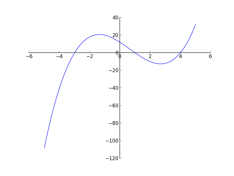
It is always a good idea to plot the function you are trying to find the root of (if possible). We can do this easily in gnuplot:

set grid
set xrange [-5:5]
plot x**3 + x**2 + 1

Here’s the implementation:

Listing 75 bisection.cpp

#include <iostream>
#include <functional>
#include <cmath>
#include <format>

namespace Roots {
    const double ATOL = 1.e-10;   // absolute tolerance
    const double RTOL = 1.e-10;   // relative tolerance
    const int MAX_ITER = 100;
}

// Apply bisection to find a root of f(x) in the range [xleft, xright]
// Return value is 0 if root found, non-zero if there was an error

int bisection(double xleft, double xright,
              std::function<double(double)> f,
              double& root) {

    int ierr{0};

    double fleft = f(xleft);
    double fright = f(xright);

    if (fleft * fright > 0) {
        std::cout << "no root in interval [xleft, right]" << std::endl;
        ierr = 1;
        return ierr;
    } else if (fleft == 0 || fright == 0) {
        std::cout << "root is one of bounds" << std::endl;
        ierr = 1;
        return ierr;
    }

    double xmid = 0.5 * (xleft + xright);

    int iter{0};

    while (iter < Roots::MAX_ITER) {
        double fmid = f(xmid);

        if (fleft * fmid > 0.0) {
            // root is in [xmid, xright]
            xleft = xmid;
            fleft = fmid;
        } else {
            // root is in [xleft, xmid]
            xright = xmid;
            // fright = fmid;  // we don't use fright
        }

        double err = std::abs(xright - xleft);
        xmid = 0.5 * (xleft + xright);

        // check if we've converged
        if (err < Roots::RTOL * std::abs(xmid) + Roots::ATOL) {
            ierr = 0;
            break;
        }

        iter++;
    }

    // check to see if we took too many iterations
    if (iter == Roots::MAX_ITER) {
        std::cout << "too many iterations" << std::endl;
        ierr = 1;
    }

    root = xmid;

    return ierr;
}

double f(double x) {
    return std::pow(x, 3.0) + std::pow(x, 2.0) - 1.0;
}

int main() {

    int ierr{0};
    double root{0.0};

    // bisection on f(x) = x^3 + x^2 - 1

    std::cout << "trying bisection on f(x) = x^3 + x^2 - 1" << std::endl;

    ierr = bisection(-5.0, 5.0, f, root);

    if (ierr == 0) {
        std::cout << std::format("x_0 = {}; f(x_0) = {}\n",
                                 root, f(root));
    } else {
        std::cout << "root not found" << std::endl;
    }
    std::cout << std::endl;

}

A few features:

• We use a namespace to hold the parameters that affect the behavior of the root finding algorithms. This ensures that if we #include another header file that defines a variable ATOL, RTOL, or MAX_ITER, that it does not clash with our versions.

  Tip

  A namespace can be used to put a number of orbits or functions into their own scope. You can then access them using the scope operator ::. This is a way to group together related concepts and makes the code easier to read.

  This is not required here, but it does help organize our code better.

• We use both a relative and absolute tolerance for assessing the error. Convergence is met when:

  \[\epsilon < \mathrm{RTOL} |x_0| + \mathrm{ATOL}\]

  This ensures that if the current estimate of the root, \(x_0\), is close to zero then \(\mathrm{ATOL}\) is used but if the root \(x_0\) is large, then \(\mathrm{RTOL}\) use used for the error.

• We have a maximum number of iterations, Roots::MAX_ITER, after which we exit with an error. This ensures we don’t get stuck in an infinite loop if something goes wrong.

Tip

It is always a good idea to plot the function you are trying to find the root of (if possible). We can do this easily in gnuplot:

set grid
set xrange [-5:5]
plot x**3 + x**2 + 1

Bisection is slow to converge—it only reduces the error by a factor of 2 each iteration.

try it…

Bisection will fail to find the root for \(f(x) = x^2\). This is because the root is tangent to the x axis—the function doesn’t change sign.

Newton’s method

For Newton’s method, we start by Taylor expanding the function about some initial guess for the root, \(x_0\):

\[f(x_0 + \delta x) \approx f(x_0) + \left . \frac{df}{dx} \right |_{x_0} \delta x + ~ ...\]

if \(x_0\) is close to the actual root, then \(\delta x\) is a correction that will bring it closer to the actual root, and the higher order terms in this expansion will be small, so we can neglect them. This tells us that the correction is:

\[\delta x = -\frac{f(x_0)}{df/dx|_{x_0}}\]

Then we can correct our guess:

\[x_0 \leftarrow x_0 + \delta x\]

and iterate on this procedure until \(|\delta x|\) is small.

Here’s an animation showing the method converging:

Important

• The initial guess needs to be good—if it is not, then the higher order terms, which start with \(\delta x^2\) are not small, and we should not have neglected them.

• We need a good estimate of the derivative. Ideally this means that we supply a function that computes the derivative analytically.

  If we don’t have an analytic form of the derivative, then we can compute it via finite-differences. This can give rise to the secant method.

Caution

Newton’s method can fail in a variety of ways, including entering a cycle. This is why we put a cap on the number of iterations.

Here’s an implementation:

Listing 76 newton.cpp

#include <iostream>
#include <functional>
#include <cmath>
#include <format>

namespace Roots {
    const double ATOL = 1.e-10;   // absolute tolerance
    const double RTOL = 1.e-10;   // relative tolerance
    const int MAX_ITER = 100;
}

// Apply Newtons's method to find a root of f(x) starting with the initial
// guess x0.  In addition to f(x) we need to supply the derivative, dfdx(x).
// Return value is 0 if root found, non-zero if there was an error

int newton(double x0,
           std::function<double(double)> f,
           std::function<double(double)> dfdx,
           double& root) {

    int ierr{1};

    int iter{0};
    while (iter < Roots::MAX_ITER ) {

        double f0 = f(x0);
        double dfdx0 = dfdx(x0);

        double dx = -f0/dfdx0;

        if (std::abs(dx) < Roots::RTOL * std::abs(x0) + Roots::ATOL) {
            ierr = 0;
            break;
        }

        x0 += dx;
        iter++;
    }

    root = x0;
    return ierr;
}

double f(double x) {
    return x * x;
}

double dfdx(double x) {
    return 2.0 * x;
}

int main() {

    std::cout << "trying Newton's method on f(x)" << std::endl;

    double root{};

    auto ierr = newton(-1.0, f, dfdx, root);

    if (ierr == 0) {
        std::cout << std::format("x_0 = {}; f(x_0) = {}\n",
                                 root, f(root));
    } else {
        std::cout << "root not found" << std::endl;
    }
    std::cout << std::endl;

}

Some notes:

• We use the same combination of a relative and absolute tolerance here as we did with bisection. Too see why, set ATOL = 0.0 for the \(f(x) = x^2\) function.

• We are not guarding against the case where \(df/dx = 0\)—this could cause problems.

  try it…

  Run the Newton method on the same problem we did for bisection:

  \[f(x) = x^3 + x^2 + 1 = 0\]

  and use an initial guess of -1. Notice that this generates an inf quickly.