Electrons and Positrons

pynucastro provides an electron-positron EOS. We will explore that here.

Warning

The ElectronEOS can be slow because it is solving for the degeneracy parameter, \(\eta\), and doing all of the integrals at high precision.

import pynucastro as pyna

import numpy as np
import matplotlib.pyplot as plt
from matplotlib import colors

Once we create an ElectronEOS, we can access the thermodynamics via the pe_state function.

es = pyna.eos.ElectronEOS()

We’ll create a grid of temperature and density and compute the thermodynamic quantities at each point.

Ts = np.logspace(4, 9, 26)
rhos = np.logspace(-4, 9, 66)

eta = np.zeros((len(rhos), len(Ts)))
n_e = np.zeros((len(rhos), len(Ts)))
n_pos = np.zeros((len(rhos), len(Ts)))

The only role composition plays in this EOS is determining the number density of electrons (assuming full ionization) via \(Y_e\).

comp = pyna.Composition(["he4"])
comp.set_equal()

for ir, rho in enumerate(rhos):
    for it, T in enumerate(Ts):
        state = es.pe_state(rho, T, comp, compute_derivs=False)
        eta[ir, it] = state.eta
        n_e[ir, it] = state.n_e
        n_pos[ir, it] = state.n_pos        

At low density and very high temperatures (\(kT \sim m_e c^2\)), we can create electron positron pairs. Here we plot the fraction of positrons to the total number of electrons and positrons.

y = (n_pos / (n_pos + n_e))
y.min(), y.max()

(np.float64(0.0), np.float64(0.499999986135348))

fig = plt.figure(constrained_layout=True)
ax = fig.add_subplot(111)
im = ax.imshow(y.T, origin="lower",
               norm=colors.SymLogNorm(linthresh=1.e-5, vmin=1.e-50, vmax=0.5, clip=True),
               extent=[np.log10(rhos.min()), np.log10(rhos.max()),
                       np.log10(Ts.min()), np.log10(Ts.max())],
               interpolation="bilinear")
ax.set_xlabel(r"$\log_{10}(\rho)$")
ax.set_ylabel(r"$\log_{10}(T)$")
ax.set_title(r"$n^+ / (n^- + n^+)$")
fig.colorbar(im, ax=ax, orientation="horizontal")

<matplotlib.colorbar.Colorbar at 0x7f7dcb2401a0>

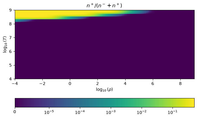
We see that we have nearly equal numbers of electrons and positrons at very low densities and high temperatures.