Stellar Evolution in the ρ-T Plane

Note

This example uses the same models as the previous example. You can download them following the instructions there.

import numpy as np
import matplotlib.pyplot as plt
import mesa_reader as mr

We’ll use a simple container to hold the models to allow us to explore them.

class Model:
    def __init__(self, mass, profiles=None, history=None):
        self.mass = mass
        if history:
            self.history = mr.MesaData(history)
        self.profiles = []
        if profiles:
            for p in profiles:
                self.profiles.append(mr.MesaData(p))

Now read in all the data. For all but the lowest mass we have 2 profiles and 1 history. The profiles were picked to roughly correspond to the midpoint of core H burning and core He burning.

models = []

models.append(Model(0.3, profiles=["M0.3_default_profile8.data"],
                    history="M0.3_default_trimmed_history.data"))

models.append(Model(1, profiles=["M1_default_profile8.data",
                                 "M1_default_profile218.data"],
                    history="M1_default_trimmed_history.data"))

models.append(Model(8, profiles=["M8_basic_co_profile8.data",
                                 "M8_basic_co_profile39.data"],
                    history="M8_basic_co_trimmed_history.data"))

models.append(Model(15, profiles=["M15_aprox21_profile8.data",
                                  "M15_aprox21_profile19.data"],
                    history="M15_aprox21_trimmed_history.data"))

HR diagram

Let’s start by looking at the models on the HR diagram and mark the location where H burning is occuring (with an \(\times\))

fig, ax = plt.subplots()

for star in models:
    ax.loglog(star.history.Teff, star.history.L,
              label=rf"{star.mass} $M_\odot$")
    ax.scatter([star.profiles[0].Teff], [star.profiles[0].photosphere_L], marker="x")

ax.legend()
ax.set_xlabel("T (K)")
ax.set_ylabel(r"L ($L_\odot$)")
ax.invert_xaxis()

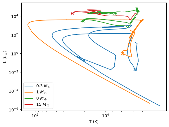
You can see the main sequence clearly on this plot.

We also see that only the 0.3 and 1 solar mass stars “finished’ stellar evolution, winding up as a cooling white dwarf at the end – the path they follow is essentially a line of constant radius, since the white dwarf does not contract as it cools (it is degenerate).

Central evolution

We want to plot the history of the evolution of the central conditions in the \(\log \rho\)-\(\log T\) plane.

We will plot the EOS boundary lines considered before. These functions are now in a module, regimes.py to make our life easier.

import regimes

Now we can plot the data

fig, ax = plt.subplots()

for star in models:
    ax.loglog(star.history.center_T, star.history.center_Rho,
              label=rf"{star.mass} $M_\odot$")

rho = np.logspace(-5, 8, 100)
ax.loglog(regimes.deg_ideal(rho, mu_e=1.3), rho, color="0.5", ls=":")
ax.loglog(regimes.rad_ideal(rho, mu=0.6), rho, color="0.5", ls=":")
ax.legend()

ax.set_xlabel(r"$T_c$ [K]")
ax.set_ylabel(r"$\rho_c$ [g/cc]")

ax.set_xlim(1.e5, 1.e9)

(100000.0, 1000000000.0)

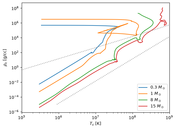
Some observations:

• The higher mass stars are closer to the line where radiation dominates.

• The 0.3 and 1 solar mass stars make a transition from following \(T \approx \rho^{1/3}\) to \(\rho = \mbox{constant}\) when degeneracy kicks in.

• The other stars more or less follow the \(T \approx \rho^{1/3}\) trend expected from polytropes + ideal gas.

We can also add approximate ignition curves, by setting

\[\epsilon = \epsilon_\mathrm{min}\]

where we use \(\epsilon_\mathrm{min} = 10^3~\mathrm{erg~g^{-1}~s^{-1}}\).

T_H = np.logspace(6.8, 7.5, 100)
rho_H = regimes.q_H(T_H)

T_He = np.logspace(7.9, 8.3, 100)
rho_He = regimes.q_He(T_He)

ax.plot(T_H, rho_H, ls="--", color="0.5")
ax.plot(T_He, rho_He, ls="--", color="0.5")

fig

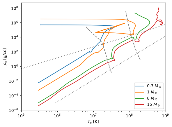
We see that the 0.3 \(M_\odot\) star never gets hot enough for He burning, while the 1.0 \(M_\odot\) star ignites He under degenerate conditions (a He flash)

Profiles

Let’s next look at the profiles of the stars in the \(\log \rho\)-\(\log T\) plane

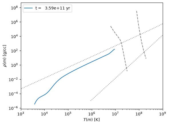
0.3 \(M_\odot\)

fig, ax = plt.subplots()

for p in models[0].profiles:
    ax.plot(p.T, p.Rho, label=f"t = {p.star_age:10.3g} yr")

ax.loglog(regimes.deg_ideal(rho, mu_e=1.3), rho, color="0.5", ls=":")
ax.loglog(regimes.rad_ideal(rho, mu=0.6), rho, color="0.5", ls=":")
ax.legend()

ax.plot(T_H, rho_H, ls="--", color="0.5")
ax.plot(T_He, rho_He, ls="--", color="0.5")

ax.set_xlabel(r"$T(m)$ [K]")
ax.set_ylabel(r"$\rho(m)$ [g/cc]")

ax.set_xlim(1.e3, 1.e9)

(1000.0, 1000000000.0)

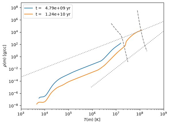
1 \(M_\odot\)

fig, ax = plt.subplots()

for p in models[1].profiles:
    ax.plot(p.T, p.Rho, label=f"t = {p.star_age:10.3g} yr")

ax.loglog(regimes.deg_ideal(rho, mu_e=1.3), rho, color="0.5", ls=":")
ax.loglog(regimes.rad_ideal(rho, mu=0.6), rho, color="0.5", ls=":")
ax.legend()

ax.plot(T_H, rho_H, ls="--", color="0.5")
ax.plot(T_He, rho_He, ls="--", color="0.5")

ax.set_xlabel(r"$T(m)$ [K]")
ax.set_ylabel(r"$\rho(m)$ [g/cc]")

ax.set_xlim(1.e3, 1.e9)

(1000.0, 1000000000.0)

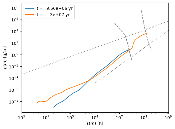
8 \(M_\odot\)

fig, ax = plt.subplots()

for p in models[2].profiles:
    ax.plot(p.T, p.Rho, label=f"t = {p.star_age:10.3g} yr")

ax.loglog(regimes.deg_ideal(rho, mu_e=1.3), rho, color="0.5", ls=":")
ax.loglog(regimes.rad_ideal(rho, mu=0.6), rho, color="0.5", ls=":")
ax.legend()

ax.plot(T_H, rho_H, ls="--", color="0.5")
ax.plot(T_He, rho_He, ls="--", color="0.5")

ax.set_xlabel(r"$T(m)$ [K]")
ax.set_ylabel(r"$\rho(m)$ [g/cc]")

ax.set_xlim(1.e3, 1.e9)

(1000.0, 1000000000.0)

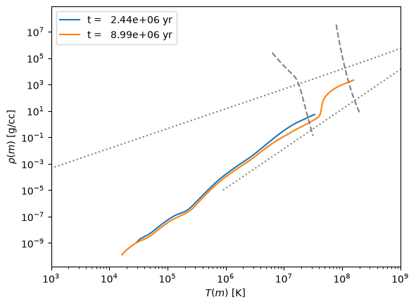
15 \(M_\odot\)

fig, ax = plt.subplots()

for p in models[3].profiles:
    ax.plot(p.T, p.Rho, label=f"t = {p.star_age:10.3g} yr")

ax.loglog(regimes.deg_ideal(rho, mu_e=1.3), rho, color="0.5", ls=":")
ax.loglog(regimes.rad_ideal(rho, mu=0.6), rho, color="0.5", ls=":")
ax.legend()

ax.plot(T_H, rho_H, ls="--", color="0.5")
ax.plot(T_He, rho_He, ls="--", color="0.5")

ax.set_xlabel(r"$T(m)$ [K]")
ax.set_ylabel(r"$\rho(m)$ [g/cc]")

ax.set_xlim(1.e3, 1.e9)

(1000.0, 1000000000.0)