p-p chain vs. CNO#
We will explore the p-p chain and the CNO cycle to learn which rates are the slowest in each and when each dominates inside of stars.
We will use pynucastro for all of this work.
import pynucastro as pyna
We start by getting the rates from the JINA ReacLib database. This has 80,000+ reaction rates in a standardized format.
rl = pyna.ReacLibLibrary()
Simple p-p chain#
We’ll start by getting the 3 main sequences that make up the p-p chain.
pp_rates = ["p(p,)d",
            "d(p,g)he3",
            "he3(he3,pp)he4"]
rates = rl.get_rate_by_name(pp_rates)
We can look at which rates it pulled in:
for r in rates:
    print(r)
p + p ⟶ H2 + e⁺ + 𝜈
p + p + e⁻ ⟶ H2 + 𝜈
H2 + p ⟶ He3 + 𝛾
He3 + He3 ⟶ p + p + He4
Note that ReacLib actually splits the p+p rate into two. We will add them together.
We can look at the temperature dependence of one of these rates
r = rates[0]
fig = r.plot(Tmin=1.e7, Tmax=1.e8)
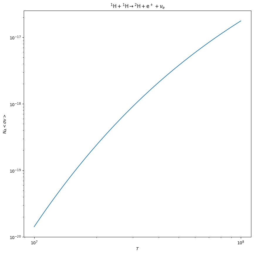
We see that it is very temperature dependent
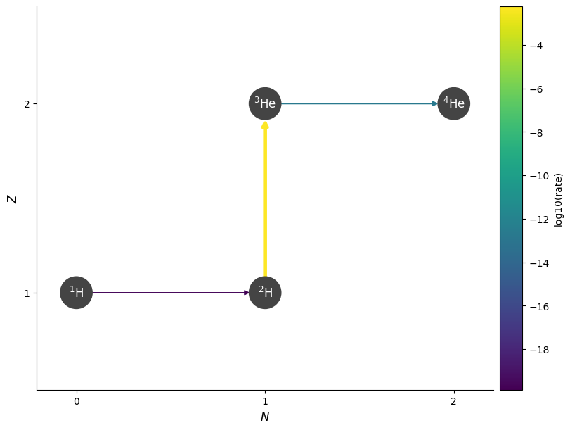
Next we build our network (we’ll use a RateCollection) with these rates
rc_pp = pyna.RateCollection(rates=rates)
We can create a thermodynamic state approximating the center of the Sun and evaluate the rates
T = 1.5e7
rho = 150
comp = pyna.Composition(rc_pp.unique_nuclei)
comp.set_solar_like()
rc_pp.evaluate_rates(rho, T, comp)
{p + p ⟶ H2 + e⁺ + 𝜈: 2.978374743269655e-18,
 p + p + e⁻ ⟶ H2 + 𝜈: 1.357778476769111e-20,
 H2 + p ⟶ He3 + 𝛾: 0.005874533290651895,
 He3 + He3 ⟶ p + p + He4: 1.849294558580789e-13}
We see from this that the first reaction, p + p, is by far the slowest.
fig = rc_pp.plot(rho=rho, T=T, comp=comp, hide_xp=True, always_show_alpha=True)
We can therefore approximate the p-p chain based on the slowest rate. If we express the rate as:
then we can find the exponent \(\nu\) about some temperature \(T_0\)
r_pp = rc_pp.get_rate_by_name("p(p,)d")[0]
T0 = 1.5e7
r_pp.get_rate_exponent(T0)
3.9735120801889896
Around the conditions in the Sun, the p-p chain has a temperature dependence of \(\sim T^4\)
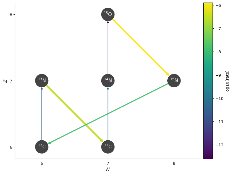
CNO#
Now we consider the main CNO cycle. This involves 6 rates
cno_rates = ["c12(p,g)n13",
             "c13(p,g)n14",
             "n13(,)c13",
             "n14(p,g)o15",
             "n15(p,a)c12",
             "o15(,)n15"]
rates = rl.get_rate_by_name(cno_rates)
for r in rates:
    print(r)
C12 + p ⟶ N13 + 𝛾
C13 + p ⟶ N14 + 𝛾
N13 ⟶ C13 + e⁺ + 𝜈
N14 + p ⟶ O15 + 𝛾
N15 + p ⟶ He4 + C12
O15 ⟶ N15 + e⁺ + 𝜈
rc_cno = pyna.RateCollection(rates=rates)
comp = pyna.Composition(rc_cno.unique_nuclei)
comp.set_solar_like()
Again we can look evaluate each of the rates:
rc_cno.evaluate_rates(rho, T, comp)
{C12 + p ⟶ N13 + 𝛾: 1.0467759242295144e-17,
 C13 + p ⟶ N14 + 𝛾: 3.176211597339995e-17,
 N13 ⟶ C13 + e⁺ + 𝜈: 2.9720852738029567e-07,
 N14 + p ⟶ O15 + 𝛾: 1.7295781984662848e-20,
 N15 + p ⟶ He4 + C12: 6.954822248932605e-16,
 O15 ⟶ N15 + e⁺ + 𝜈: 1.2625681768893481e-06}
Now we see that the N14(p,g)O15 rate is the slowest.
r_cno = rc_cno.get_rate_by_name("n14(p,g)o15")
This is a much steeper function of temperature. Let’s explore the temperature dependence around a few points
for T in [1.e7, 2.e7, 3.e7, 4.e7]:
    print(f"T = {T}, nu = {r_cno.get_rate_exponent(T)}")
T = 10000000.0, nu = 22.829615097171867
T = 20000000.0, nu = 17.966372387768573
T = 30000000.0, nu = 15.601859314950396
T = 40000000.0, nu = 14.115346885210606
Here’s what the CNO cycle looks like
fig = rc_cno.plot(rho=rho, T=T, comp=comp, hide_xp=True)
Comparing p-p vs. CNO#
The temperature dependence suggests that if the temperature were a little higher, then CNO would go faster then p-p. We can plot the two rate-limiting rates on the same axes
import numpy as np
import matplotlib.pyplot as plt
Ts = np.logspace(6.8, 8, 50)
fig, ax = plt.subplots()

ax.plot(Ts, [r_pp.eval(q) for q in Ts], label="p-p")
ax.plot(Ts, [r_cno.eval(q) for q in Ts], label="CNO")
ax.set_xscale("log")
ax.set_yscale("log")
ax.grid(linestyle=":", which="both")
ax.legend()
<matplotlib.legend.Legend at 0x7f59cf3b9c40>
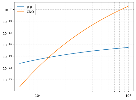
Notice that they cross over at a temperature just hotter than the Sun’s core. This means that stars more massive than the Sun (actually, about \(1.5~M_\odot\)) are powered by CNO and less massive stars are powered by p-p. The strong \(T\) dependence of CNO will play a role in determining the structure of those more massive stars.