Nuclear statistical equilibrium

import pynucastro as pyna

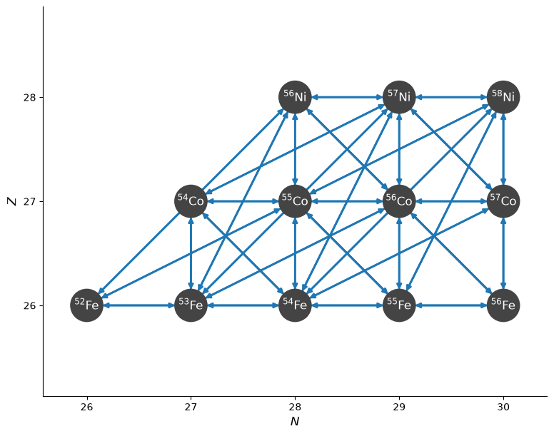
We’ll explore only a small set of nuclei around the iron-group. Of course, nature can access all nuclei, so our results will be an approximation.

The NSE abundance depends on \((\rho, T, Y_e)\). In particular, the electron fraction, \(Y_e\) is going to dictact the electron fraction of the resulting NSE composition.

rlib = pyna.ReacLibLibrary()
nse_lib = rlib.linking_nuclei(["p", "n", "he4",
                               "fe52", "fe53", "fe54", "fe55", "fe56",
                               "co54", "co55", "co56", "co57",
                               "ni56", "ni57", "ni58"])

nse = pyna.NSENetwork(libraries=nse_lib)

fig = nse.plot()

Let’s start with some conditions that are roughly appropriate for the core of a massive star.

We’ll start with \(Y_e = 0.5\) and then see how the composition changes as it is lowered.

rho = 1.e9
T = 6.e9
Ye = 0.5

comp = nse.get_comp_nse(rho, T, Ye, use_coulomb_corr=True)
fig = comp.plot()

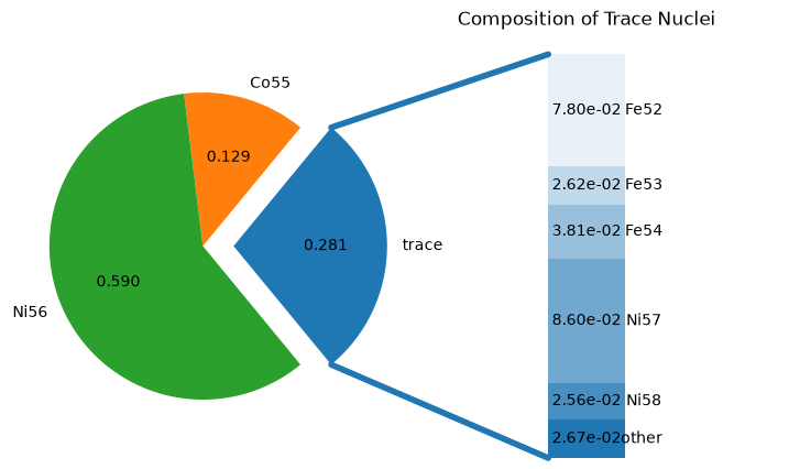
Here we see that \({}^{56}\mathrm{Ni}\) dominates, as expected since \(Z/A\) for it is 1/2.

Now let’s lower Ye

Ye = 0.49
comp = nse.get_comp_nse(rho, T, Ye, use_coulomb_corr=True)
fig = comp.plot()

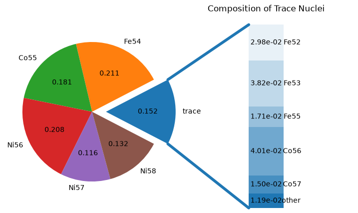
Now we see that some neutron-rich nuclei start to appear in large abundance.

Let’s lower again.

Ye = 0.47
comp = nse.get_comp_nse(rho, T, Ye, use_coulomb_corr=True)
fig = comp.plot()

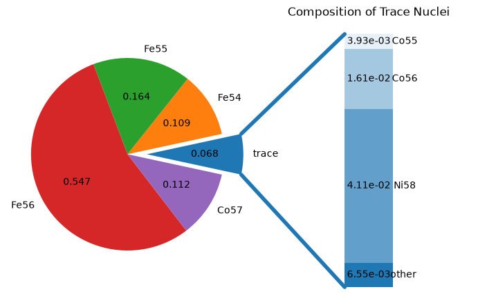
\({}^{56}\mathrm{Fe}\) has \(Z/A = 0.464\), so as we drop \(Y_e\) down to that level, we see it starting to dominate.

Trend with temperature

Let’s look at a fixed \(Ye\) how the composition changes. We’ll do \(Y_e = 0.48\).

import numpy as np
import matplotlib.pyplot as plt

We use the chemical potentials from the previous solve to help accelerate the next solve.

ye = 0.48
temps = np.logspace(9, 10.5, 100)
X_s = []
T_s = []
guess = [-3.5, -15.0]
for T in reversed(temps):
    nse_comp, sol = nse.get_comp_nse(rho, T, ye, init_guess=guess,
                                     use_coulomb_corr=True, return_sol=True)
    guess = sol
    nse_X_s = [nse_comp.X[nuc] for nuc in nse_comp.X]
    T_s.append(T)
    X_s.append(nse_X_s)

X_s = np.array(X_s)
nuc_names = nse.get_nuclei()

low_limit = 0.05
fig, ax = plt.subplots()
for k in range(len(nuc_names)):
    line, = ax.plot(T_s, X_s[:,k])
    if (max(X_s[:,k]) > low_limit):
        line.set_label(str(nuc_names[k]))
    if (max(X_s[:,k]) > 5 * low_limit):
        line.set_linewidth(2.5)

ax.legend(ncols=3, fontsize="small")
ax.set_xlabel(r"temperature $[K]$")
ax.set_ylabel("mass Fraction")
ax.set_xscale("log")
ax.set_yscale("log")
ax.set_ylim([low_limit, 1.2])
ax.grid(ls=":")

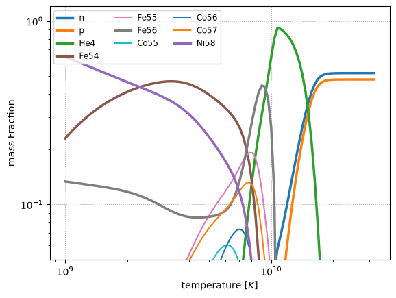
We see that at very high temperatures, the composition goes to mostly \(\alpha\) first and then to a mix of neutrons and protons.